Modelling Structured Noise • genpca

The problem

Real data rarely offers a clean choice. An fMRI run has smooth signal (distributed networks), smooth noise (drift, vascular and physiological fluctuation), rough noise (thermal), and sometimes rough signal (focal activation, tissue boundaries) — all at once. The obvious question is which metric to reach for, and the honest answer is that the choice is better-defined than it looks in some cases and impossible in others.

This vignette works out which is which. Every number below is produced by the code shown.

A metric is a spectral filter

Build a graph over your variables — voxels adjacent in space, time points adjacent in a series — and take its Laplacian $L$ . The eigenvectors of $L$ are a Fourier basis for that graph: small eigenvalues are smooth patterns, large eigenvalues are rough ones. Then any metric of the form

$A = f(L) = \sum_j f(\lambda_j)\,\phi_j\phi_j^{\top}$

is a filter, and $f$ is its transfer function. This covers the Laplacian-based filters compared below; general metrics need not share this graph’s eigenvectors.

g <- 12; p <- g * g; n <- 150
gi <- expand.grid(r = 1:g, c = 1:g)
W <- matrix(0, p, p)
for (i in 1:p) for (j in 1:p)
  if (i < j && abs(gi$r[i] - gi$r[j]) + abs(gi$c[i] - gi$c[j]) == 1) {
    W[i, j] <- 1; W[j, i] <- 1
  }
L  <- diag(rowSums(W)) - W
eL <- eigen(L, symmetric = TRUE)
Q  <- eL$vectors
lam <- pmax(eL$values, 0)

# build a metric from a transfer function of the Laplacian
spec <- function(f) Q %*% (f(lam) * t(Q))

Note that eigen() returns eigenvalues in decreasing order, so Q[, 1] is the roughest graph mode and Q[, p] the smoothest. Getting this backwards is an easy way to convince yourself of something false.

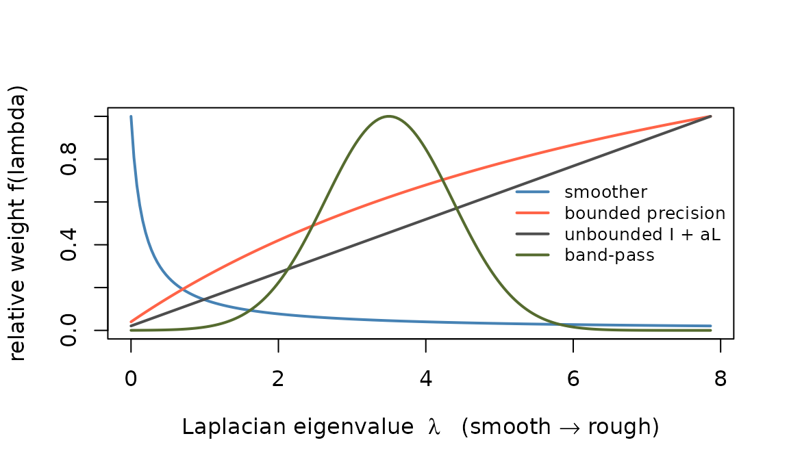
Four transfer functions on the same graph, each normalized to a maximum of one. Lower Laplacian eigenvalues represent smoother patterns; there is no single boundary between smooth and rough.

So the practical vocabulary is not “adjacency versus Laplacian” — those are just two points on this continuum. You are choosing a curve.

Building these matrices in practice

You rarely have to assemble a graph by hand. The adjoin package constructs weighting matrices from coordinates or from the data itself, and supplies both orientations directly: spatial_adjacency(), spatial_smoother(), heat_kernel() and graph_weights() on the smoother side; spatial_laplacian() and temporal_laplacian() on the precision side, with temporal_adjacency() for the time margin.

cds  <- as.matrix(expand.grid(x = 1:8, y = 1:8))
Aadj <- adjoin::spatial_adjacency(cds, nnk = 8, weight_mode = "heat", sigma = 1.5)
Alap <- adjoin::spatial_laplacian(cds, nnk = 8, weight_mode = "heat", sigma = 1.5)

# check the two traps before using either as a metric
range(eigen(as.matrix(Aadj), symmetric = TRUE, only.values = TRUE)$values)
#> [1] -0.1882372  1.0065493
range(eigen(as.matrix(Alap), symmetric = TRUE, only.values = TRUE)$values)
#> [1] 4.676095e-16 1.490016e+00

Both traps from the previous section show up in real output. The adjacency comes back indefinite — its smallest eigenvalue is negative, so it is not a metric until you shift it (Aadj + c * Diagonal(n), or repair_metric(Aadj, method = "ridge"), which also reports how large the shift had to be); genpca() refuses it as supplied unless you opt into a repair with constraints_remedy. The Laplacian comes back PSD but exactly singular, its null vector being the spatially constant pattern; genpca() accepts that via a pseudo-inverse, but Alap + eps * Diagonal(n) is usually what you want. Neither is a defect in adjoin — an adjacency matrix simply is not positive definite, and that is a property of graphs, not of the software.

With those repairs, the two point in the directions their spectral orientations predict: used as a column metric, the adjacency produces markedly smoother loadings than plain PCA and the Laplacian markedly rougher ones.

What a metric can and cannot separate

A metric of the form $f(L)$ reweights graph frequencies. It can favour frequencies with a better signal-to-noise ratio, but cannot distinguish signal and noise contributions within the same graph mode.

We plant a signal of known spatial character in noise of known spatial character, and measure how well the leading component recovers it.

nrm  <- function(v) v / sqrt(sum(v^2))
# how much of the planted pattern is captured by the fitted subspace?
recov <- function(V, truth) {
  V <- qr.Q(qr(as.matrix(V)))
  sqrt(sum((t(V) %*% truth)^2)) / sqrt(sum(truth^2))
}

smooth_pat <- nrm(exp(-((gi$r - 4)^2 + (gi$c - 4)^2) / 6))     # a blob
fine_pat   <- nrm(Q[, which.min(abs(lam - median(lam)))])      # a mid-frequency mode

smooth_noise <- function(n) {
  Z <- matrix(rnorm(n * p), n, p) %*% spec(function(l) sqrt(1 / (1 + 4 * l)))
  Z / sqrt(mean(Z^2))
}
fine_noise <- function(n) {
  Z <- matrix(rnorm(n * p), n, p) %*% spec(function(l) sqrt((l + .5) / max(lam)))
  Z / sqrt(mean(Z^2))
}

A_smoother  <- spec(function(l) 1 / (1 + 6 * l))
A_precision <- spec(function(l) 1 / (0.02 + 1 / (1 + 6 * l)))

set.seed(909)
reps <- 8
grid <- expand.grid(signal = c("smooth", "fine"), noise = c("smooth", "fine"),
                    stringsAsFactors = FALSE)
out <- t(apply(grid, 1, function(row) {
  pat <- if (row[["signal"]] == "smooth") smooth_pat else fine_pat
  acc <- c(0, 0, 0)
  for (r in seq_len(reps)) {
    E <- if (row[["noise"]] == "smooth") smooth_noise(n) else fine_noise(n)
    X <- scale(matrix(rnorm(n), n, 1) %*% t(pat) * 1.1 + E, scale = FALSE)
    for (k in 1:3) {
      A <- list(diag(p), A_smoother, A_precision)[[k]]
      fit <- genpca(X, A = A, ncomp = 1, preproc = multivarious::pass())
      acc[k] <- acc[k] + recov(fit$ov, pat) / reps
    }
  }
  acc
}))
dimnames(out) <- list(paste(grid$signal, "signal /", grid$noise, "noise"),
                      c("identity", "smoother", "precision"))
round(out, 3)
#>                              identity smoother precision
#> smooth signal / smooth noise    0.437    0.495     0.336
#> fine signal / smooth noise      0.031    0.023     0.573
#> smooth signal / fine noise      0.058    0.733     0.035
#> fine signal / fine noise        0.144    0.200     0.063

In these simulations, matching the metric to the spectral contrast makes a large difference: the smoother helps the smooth signal in fine noise, while the precision helps the fine signal in smooth noise. The other metric can perform worse than identity. These are averages over eight simulated data sets, not accuracy guarantees for a new data set.

When signal and noise have the same broad label, the gains are smaller and the rankings vary. A broad label such as “smooth” does not imply identical spectra, so it cannot establish that no filter could help. If signal and noise have identical spectral profiles, however, reweighting those profiles cannot improve their relative power.

Planted signal	Noise	Result among these three metrics
Smooth	Fine	Large gain with the smoother
Fine	Smooth	Large gain with the precision
Smooth	Smooth	Smaller differences; no comparable gain
Fine	Fine	Smaller differences; ranking depends on the filter

For a mixture of signal and nuisance structures, estimate where their spectral profiles differ. The table describes the constructed examples; it is not a decision rule based solely on the words “smooth” and “fine”.

Whiten by the noise, not by the signal

The rule for choosing $f$ follows from the model rather than from taste. Under separable noise, $A = \Sigma_{\text{col}}^{-1}$ makes GPCA the maximum-likelihood low-rank fit, so the metric is determined by the noise, whatever the signal happens to look like.

For a realistic two-component noise model — smooth physiological fluctuation plus broadband thermal noise —

$\Sigma_{\text{col}} = \sigma_s^2\,K + \sigma_r^2 I \qquad\Longrightarrow\qquad A = \left(\sigma_s^2\,K + \sigma_r^2 I\right)^{-1},$

which is the “bounded precision” curve in the first figure. It suppresses the smooth band where the physiological noise lives and then flattens out at $1/\sigma_r^2$ instead of growing without limit. Two knobs, both with physical meaning, both estimable from resting or baseline data.

Estimate them from data that does not contain your effect — a baseline run, or the residuals after removing the design — rather than from the data you are about to decompose.

Compare bounded and linearly increasing weights

The noise-floor term changes the high-frequency behaviour: an unbounded metric such as $I + \alpha L$ keeps increasing with $\lambda$ , so it places its largest weight on the very roughest directions. Broadband thermal noise is present there too; whether those directions contain useful signal depends on the application.

A_unbounded <- spec(function(l) 1 + 6 * l)

set.seed(78)
acc <- c(0, 0, 0); reps <- 8
for (r in seq_len(reps)) {
  X <- scale(matrix(rnorm(n), n, 1) %*% t(fine_pat) * 1.1 +
             smooth_noise(n) * 0.8 +
             matrix(rnorm(n * p), n, p) * 0.8, scale = FALSE)   # + thermal
  for (k in 1:3) {
    A <- list(diag(p), A_precision, A_unbounded)[[k]]
    fit <- genpca(X, A = A, ncomp = 1, preproc = multivarious::pass())
    acc[k] <- acc[k] + recov(fit$ov, fine_pat) / reps
  }
}
setNames(round(acc, 3), c("identity", "bounded precision", "unbounded I + 6L"))
#>          identity bounded precision  unbounded I + 6L 
#>             0.042             0.552             0.456

Both precisions improve recovery in this example, with a modest advantage for the bounded form. It follows from the stated smooth-plus-broadband noise model, rather than from a general guarantee that bounded filters always win. Here “unbounded” describes the function as its argument grows; on this finite graph, I + 6L has a finite largest eigenvalue. Neither curve alone supplies a worst-case guarantee for statistical recovery.

Use both margins

Signal and noise with overlapping spatial profiles may differ in time. A task response and drift can, for example, occupy different temporal bands. That is what the row metric is for, and it is why M and A are separate arguments rather than one blended constraint.

Here the noise is temporally autocorrelated, the signal is task-locked at a frequency where that noise has little power, and the row metric is the AR(1) precision — the same prewhitening used in a standard fMRI GLM.

rho   <- 0.85
Sig_t <- outer(0:(n - 1), 0:(n - 1), function(i, j) rho^abs(i - j))
M_ar  <- solve(Sig_t + 1e-6 * diag(n))
task  <- scale(sin(2 * pi * (1:n) / 7))

set.seed(303)
acc <- c(0, 0); reps <- 8
for (r in seq_len(reps)) {
  E <- t(chol(Sig_t)) %*% matrix(rnorm(n * p), n, p)      # AR(1) in time
  X <- scale(task %*% t(smooth_pat) + E, scale = FALSE)
  acc[1] <- acc[1] + recov(genpca(X, ncomp = 1,
                                  preproc = multivarious::pass())$ov, smooth_pat) / reps
  acc[2] <- acc[2] + recov(genpca(X, M = M_ar, ncomp = 1,
                                  preproc = multivarious::pass())$ov, smooth_pat) / reps
}
setNames(round(acc, 3), c("no row metric", "AR(1) precision M"))
#>     no row metric AR(1) precision M 
#>             0.069             0.733

Roughly a tenfold improvement on the same data, with the column metric left as identity throughout. In this construction, temporal weighting exposes the planted pattern without specifying a spatial metric.

The practical consequence for imaging: put temporal nuisances on M (AR prewhitening, down-weighting motion-corrupted frames) and spatial nuisances on A, and regress out what is better removed by design — drift terms, physiological regressors — before decomposing at all.

When one metric is not enough

A single $A = f(L)$ applies the same spectral weighting to every component. If different components need different treatment, fitting one shared metric may be too restrictive.

sfpca() selects sparsity penalties per component, allowing different spatial supports. Its spatial roughness operator is built from spat_cds, with strength controlled by alpha_v; this is not an arbitrary per-component spectral filter.

The experimental gpca_mle() and mnpca_mrl() instead estimate a shared M and A by penalized maximum likelihood, the latter with sparse precision matrices. They reduce the need to specify those metrics in advance, but do not remove the restriction to one metric pair for the fit.

Caveats worth carrying

Separability is an approximation. The matrix-normal interpretation assumes noise covariance factorizes as $\Sigma_{\text{space}} \otimes \Sigma_{\text{time}}$ . This can be a useful approximation for independent noise or fixed spatial smoothing. Mixtures of spatially localized physiological sources with different temporal profiles can violate it. The algebraic decomposition still exists when separability fails, but that noise-likelihood interpretation no longer follows.

Whitening does not create signal. Equalizing the noise floor changes which directions dominate the decomposition; it does not change the signal-to-noise ratio within any direction. A signal below the noise in its own band stays below it.

Validate on your own data. Every number here comes from a simulation whose ground truth we chose. Sweep the strength of your metric, look at the loadings, and confirm the components move the way you expect before believing a result that depends on the metric.

Where next

GPCA Metrics — concrete recipes and the smoother/precision orientation rule.
Getting Started — the decomposition itself, and what the metrics mean geometrically.
GPCA at Scale — backends for when these metrics get large.