Sparse and Functional PCA with sfpca() • genpca

sfpca() estimates principal components that are sparse and smooth at the same time. Ordinary PCA gives you loadings that are dense — every variable loads on every component — and that spread noise across the whole map. If you know your variables live somewhere (voxels on a grid, sensors in a room, wavelengths along a spectrum) and that the real signal is localised and spatially coherent, you can ask for both properties directly.

The two requests pull in different directions, which is the point. Sparsity alone gives you a scatter of isolated survivors; smoothness alone gives you a blurred map with no zeros anywhere. Together they give compact regions with soft edges.

When to reach for it

Use sfpca() when both of these hold:

The loadings should be mostly zero — only a minority of variables participate in any given component.
The non-zero part should be coherent in some known geometry — neighbours should resemble each other.

If you only want structure and not sparsity, genpca() with a smoothing metric is the simpler tool; see GPCA Metrics. If you want sparsity with no geometry, an ordinary sparse PCA will do. sfpca() is for the case where you want both, and it is worth knowing that it reaches them by a different mechanism than genpca() — see Metric form versus constraint form below, because the two take opposite inputs for the same intent.

A worked example

Two spatially localised signals on a 16 × 16 grid, each modulated by its own temporal profile, buried in noise. The spatial patterns are Gaussian bumps truncated to zero away from their centres, so they are genuinely sparse (29 of 256 locations) and smooth on their support:

set.seed(11)
g <- 16; p <- g * g; n <- 64
gr <- expand.grid(r = 1:g, c = 1:g)

# NOTE the orientation: spatial dimensions in ROWS, variables in COLUMNS
spat_cds <- rbind(gr$r, gr$c)
dim(spat_cds)
#> [1]   2 256

blob <- function(r0, c0, s = 1.6) {
  z <- exp(-((gr$r - r0)^2 + (gr$c - c0)^2) / (2 * s^2))
  z[z < 0.15] <- 0                       # compact support => sparse
  z / sqrt(sum(z^2))
}
v1 <- blob(5, 5); v2 <- blob(12, 12)

tt <- (0:(n - 1)) / n                    # orthogonal temporal profiles
u1 <- sin(2 * pi * tt); u1 <- u1 / sqrt(sum(u1^2))
u2 <- sin(4 * pi * tt); u2 <- u2 / sqrt(sum(u2^2))

signal <- 30 * tcrossprod(u1, v1) + 20 * tcrossprod(u2, v2)
X <- signal + matrix(rnorm(n * p, sd = 0.25), n, p)

c(true_support = sum(v1 != 0), of = p,
  SNR = round(norm(signal, "F") / norm(X - signal, "F"), 2))
#> true_support           of          SNR 
#>        29.00       256.00         1.13

The Frobenius signal-to-noise ratio is 1.13. This ratio describes total matrix energy; it does not by itself determine the difficulty of recovering a leading component. Fit two components:

fit <- sfpca(X, K = 2, spat_cds = spat_cds)
fit
#> Sparse Functional PCA (sfpca)
#>   components: 2 
#>   dims: 64 obs x 256 vars
#>   singular values: 29.97, 20.31 
#>   verbs: scores(), components(), sdev(), reconstruct()

With the default penalties, BIC selects the sparsity level for each component:

V <- multivarious::components(fit)
c(nonzero_PC1 = sum(V[, 1] != 0), nonzero_PC2 = sum(V[, 2] != 0), of = p)
#> nonzero_PC1 nonzero_PC2          of 
#>          31          29         256

Against the truth, and against ordinary PCA on the same matrix:

pc <- prcomp(as.matrix(X), center = TRUE, rank. = 2)

rbind(
  sfpca = c(PC1 = abs(cor(V[, 1], v1)),        PC2 = abs(cor(V[, 2], v2))),
  pca   = c(PC1 = abs(cor(pc$rotation[, 1], v1)), PC2 = abs(cor(pc$rotation[, 2], v2)))
)
#>             PC1       PC2
#> sfpca 0.9974423 0.9934027
#> pca   0.9918938 0.9823328

Correlation alone barely separates them — PCA finds where the signal is perfectly well. The difference is everything else: PCA has to spend all 256 loadings to say it, so the map carries a noise floor everywhere the true pattern is zero.

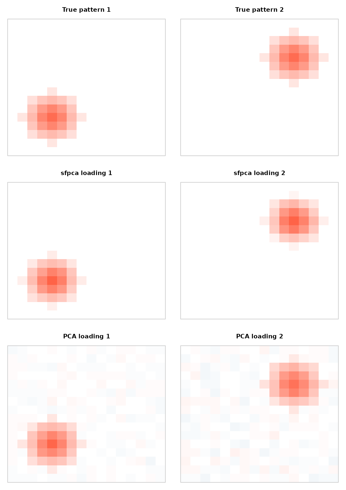
Truth, sfpca, and PCA with signs aligned to truth and one common color scale: blue is negative, white is zero, red is positive. sfpca has a few extra nonzero sites in PC1; PCA has nonzero loadings throughout.

The temporal factors are recovered too — those are the ou slot, penalised for roughness along the row index:

U <- fit$ou
c(PC1 = abs(cor(U[, 1], u1)), PC2 = abs(cor(U[, 2], u2)))
#>       PC1       PC2 
#> 0.9985844 0.9943258

The selected supports have 31 and 29 sites, compared with 29 in each planted pattern. Sparsity removes much of the off-pattern noise, although support recovery is not exact. Measured against the noiseless signal:

Xhat  <- as.matrix(multivarious::reconstruct(fit))
pchat <- pc$x %*% t(pc$rotation) + matrix(pc$center, n, p, byrow = TRUE)

c(sfpca = norm(signal - Xhat,  "F") / norm(signal, "F"),
  pca   = norm(signal - pchat, "F") / norm(signal, "F"))
#>     sfpca       pca 
#> 0.1129105 0.2014448

What the two penalties do

Each factor carries two penalties, and they are worth separating in your head. For the column factor v those are lambda_v (sparsity) and alpha_v (smoothness); lambda_u and alpha_u do the same for the row factor u. Switching each off in turn shows which is responsible for what:

variants <- list(
  "defaults"                  = list(),
  "no sparsity (lambda_v = 0)" = list(lambda_v = 0),
  "no smoothing (alpha_v = 0)" = list(alpha_v = 0),
  "neither"                    = list(lambda_v = 0, alpha_v = 0),
  "heavy sparsity (lambda_v = 3)" = list(lambda_v = 3)
)

t(sapply(variants, function(extra) {
  f <- do.call(sfpca, c(list(X = X, K = 1, spat_cds = spat_cds), extra))
  v <- multivarious::components(f)[, 1]
  c(nonzero = sum(v != 0), cor_with_truth = round(abs(cor(v, v1)), 3))
}))
#>                               nonzero cor_with_truth
#> defaults                           31          0.997
#> no sparsity (lambda_v = 0)        256          0.992
#> no smoothing (alpha_v = 0)         29          0.995
#> neither                           256          0.992
#> heavy sparsity (lambda_v = 3)      21          0.955

Sparsity is what produces the zeros: drop lambda_v and all 256 sites load. Smoothness does not create zeros — it decides which sites survive and keeps the surviving map coherent. And sparsity can be overdone: at lambda_v = 3 the support is cut below the true 29 sites and the recovered pattern degrades.

Choosing the penalties

Both kinds of penalty have defaults you can usually leave alone.

Sparsity (lambda_u, lambda_v). Left NULL, each is chosen per component by a BIC-style criterion along a regularisation path — nlambda values log-spaced down from a closed-form lambda_max, warm-started. The all-zero solution is a legitimate candidate: a component with no support worth its degrees of freedom comes back exactly zero with d = 0, which is a feature, not a failure. Fix the value explicitly to bypass the search.

Smoothness (alpha_u, alpha_v). Left NULL, each defaults to $1/\lambda_{\max}(\Omega)$ , so the roughest direction of the penalty is weighted exactly as strongly as the identity term. That makes the default invariant to how you scaled Omega and bounds the condition number of every inner solve by 2.

What was selected is stored on the fit:

data.frame(
  component = 1:2,
  lambda_u  = signif(fit$lambda_u, 3), lambda_v = signif(fit$lambda_v, 3),
  alpha_u   = signif(fit$alpha_u, 3),  alpha_v  = signif(fit$alpha_v, 3)
)
#>   component lambda_u lambda_v alpha_u alpha_v
#> 1         1   0.0891    0.859  0.0626   0.204
#> 2         2   0.2950    0.912  0.0626   0.204

The penalty shape is set by penalty_u / penalty_v: "l1" (the default) or "scad". SCAD applies less shrinkage to large coefficients, so surviving loadings keep more of their magnitude, at the price of a non-convex subproblem.

Reading the output

sfpca() returns a bi_projector, so the usual multivarious verbs work: scores() for $UD$ , components() for the sparse loadings $V$ , sdev() for $d_k$ , and reconstruct(). Two things about it differ from genpca() and will bite if you assume otherwise.

The example above is too well behaved to show either, which is itself worth knowing: its two components were built orthogonal, so they come out very nearly orthogonal and the pitfalls stay hidden. Refit on data whose components share a temporal profile, and both surface:

u2c <- sin(2 * pi * tt + 0.9); u2c <- u2c / sqrt(sum(u2c^2))
round(sum(u1 * u2c), 3)                 # the two profiles now overlap
#> [1] 0.622

set.seed(11)
Xc  <- 30 * tcrossprod(u1, v1) + 20 * tcrossprod(u2c, v2) +
       matrix(rnorm(n * p, sd = 0.25), n, p)
fc  <- sfpca(Xc, K = 2, spat_cds = spat_cds)
Uc  <- fc$ou; Vc <- multivarious::components(fc)

The factors are not orthogonal. Each rank-1 term comes from its own constraint-form subproblem rather than a joint SVD. Columns are unit-norm, but $U^{\top}U \ne I$ and $V^{\top}V \ne I$ in general:

round(crossprod(Uc), 3)     # would be the identity for a joint SVD
#>        PC1    PC2
#> PC1  1.000 -0.128
#> PC2 -0.128  1.000
round(crossprod(Vc), 3)
#>        PC1    PC2
#> PC1  1.000 -0.133
#> PC2 -0.133  1.000

sdev() is not the singular values of X. It is the covariance each component captures, $d_k = u_k^{\top} X_k v_k$ , where $X_k$ is the matrix after the previous components have been deflated out. Only the first component is measured against the original data:

Xm   <- as.matrix(Xc)
dc   <- multivarious::sdev(fc)
defl <- Xm - dc[1] * tcrossprod(Uc[, 1], Vc[, 1])

c(sdev_2      = dc[2],
  u2_X_v2     = as.numeric(t(Uc[, 2]) %*% Xm   %*% Vc[, 2]),   # does NOT match
  u2_Xdefl_v2 = as.numeric(t(Uc[, 2]) %*% defl %*% Vc[, 2]))   # matches
#>      sdev_2     u2_X_v2 u2_Xdefl_v2 
#>    13.93150    14.49848    13.93150

The gap is small here but it is not noise, and it grows with how much the components share. Treat sdev() as “covariance captured by this component given the previous ones”, never as a singular value of X.

Because $V$ is not orthogonal, reconstruct() multiplies the stored factors directly as $UDV^{\top}$ rather than going through pseudo-inverse identities, which would not reproduce the fitted model.

Metric form versus constraint form

This is the trap when moving between sfpca() and genpca(): they take opposite inputs for the same intent.

In genpca(), the structure matrix $A$ is a metric, and a metric amplifies its own dominant eigendirections — the loadings are $AV$ . To get smooth loadings you pass a smoother (a PSD kernel, an adjacency shifted to be PSD, $(I + \alpha\Omega)^{-1}$ ).

In sfpca(), the same information enters as a constraint, $v^{\top}(I + \alpha\Omega)v \le 1$ , which charges rough $v$ against a fixed budget. So you supply the roughness operator directly, and a larger alpha_v means a smoother result.

	`genpca()`	`sfpca()`
Structure enters as	metric $A$	constraint $v^{\top}(I+\alpha\Omega)v \le 1$
For smooth loadings, supply	a smoother (kernel, $(I+\alpha\Omega)^{-1}$ )	a roughness operator ( $\Omega$ , a Laplacian)
Turning the knob up	amplifies $A$ ’s top directions	smooths more

The same Laplacian therefore smooths in sfpca() and roughens in genpca(). GPCA Metrics works through the metric-side version of this in detail.

Practical notes

spat_cds is dimensions × variables. Rows are spatial axes, columns are variables, so ncol(spat_cds) must equal ncol(X). This is the transpose of the layout a coordinate data frame usually has, and it is the easiest thing to get wrong here — so the shape is checked up front:

sfpca(X, K = 1, spat_cds = t(spat_cds))
#> Error in `sfpca()`:
#> ! `spat_cds` must have one column per variable: ncol(X) is 256 but ncol(spat_cds) is 2. It looks transposed -- `spat_cds` is dimensions x variables, so pass t(spat_cds).

For a one-dimensional axis — a spectrum, a transect, a genome position — pass matrix(coords, nrow = 1) rather than a bare vector.

The column penalty is built for you. Omega_v is constructed internally from spat_cds via a knn nearest-neighbour graph (default min(6, ncol(X) - 1)); there is no Omega_v argument. Omega_u can be supplied, and defaults to a second-difference operator — which assumes the rows are ordered, as with a time series. If your rows are unordered samples, pass alpha_u = 0 rather than smoothing along a meaningless axis.

Components are extracted by deflation, so cost grows linearly in K and later components are fit to residuals. Ask for the number you intend to interpret.

Where next

GPCA Metrics covers the metric-side treatment of the same structural ideas, including how to build kernels, Laplacians and graph penalties. Modelling Structured Noise discusses choosing between them when several kinds of structure are present at once.

Reference

Allen, G. I., & Weylandt, M. (2019). Sparse and functional principal components analysis. In 2019 IEEE Data Science Workshop (DSW) (pp. 11–16). doi:[10.1109/DSW.2019.8755778](https://doi.org/10.1109/DSW.2019.8755778). Also available as arXiv:1309.2895, first posted in 2013 and revised through 2019 — the preprint and the DSW paper are the same work, which is why the literature cites both years.