Getting Started with fmrismooth

The goal of fmrismooth is to make practical, edge‑preserving smoothing and denoising easy to apply to fMRI volumes and time series. The package brings together fast lattice bilateral filters, robust and TV‑based denoisers, MP‑PCA, and simple VST wrappers, with functions that accept plain numeric arrays and optionally integrate with neuroim2 if you work with NeuroVol/NeuroVec objects. The examples below use small synthetic arrays to keep the vignette self‑contained and fast to run.

Quick start: one‑liner pipeline

The most convenient entry point is fmrismooth_default(), which infers reasonable parameters from the data and optionally runs a robust stage before a joint bilateral final stage.

library(fmrismooth)
library(ggplot2)

# helper to build a data.frame for a spatial slice (4D)
slice_df4d <- function(arr, z, t, label) {
  stopifnot(length(dim(arr)) == 4L)
  nx <- dim(arr)[1]; ny <- dim(arr)[2]
  df <- expand.grid(x = seq_len(nx), y = seq_len(ny))
  df$val <- as.vector(arr[,,z,t])
  df$method <- label
  df
}

dims <- c(8, 8, 8, 12)
clean <- array(100, dim = dims)
noisy <- clean + array(rnorm(prod(dims), sd = 4), dim = dims)

# One-liner with auto-parameters and joint bilateral final stage
smoothed <- smooth_auto(noisy, robust = "none", auto_params = TRUE)

c(var_original = var(as.vector(noisy)),
  var_smoothed  = var(as.vector(smoothed)))
#> var_original var_smoothed 
#>     16.64967     13.54920

# visualize mid-slice of a mid-frame
zmid <- ceiling(dims[3]/2); tmid <- ceiling(dims[4]/2)
viz <- rbind(
  slice_df4d(noisy, zmid, tmid, "noisy"),
  slice_df4d(smoothed, zmid, tmid, "smoothed")
)
ggplot(viz, aes(x, y, fill = val)) +
  geom_raster() +
  scale_fill_gradient(low = "black", high = "white") +
  coord_fixed() +
  scale_y_reverse() +
  facet_wrap(~method) +
  theme_minimal(base_size = 10) +
  labs(title = "Mid-slice, mid-frame", x = NULL, y = NULL, fill = "intensity")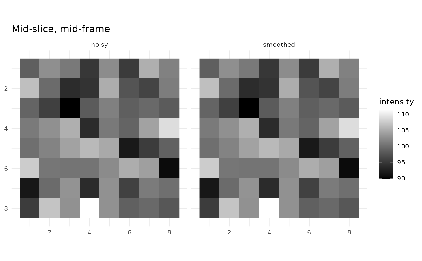

The default pipeline estimates spatial/temporal bandwidths and noise scale from the data, then applies design‑aware joint bilateral smoothing across space and time. If you have a T1 or probability maps, pass them as guides; otherwise the spatial mean of the current estimate serves as a weak guide. Note that range smoothing (sigma_r) only has an effect when a guide (or guides) is supplied — without a guide the filter is purely spatial.

MP‑PCA + joint bilateral

For stronger denoising while preserving structure, combine MP‑PCA with joint bilateral filtering using fmrismooth_mppca_pipeline().

mp_out <- smooth_mppca(
  noisy,
  sigma_mode = "global",   # estimate one sigma from temporal differences
  sigma_sp   = 2.5,
  sigma_t    = 0.5,
  sigma_r    = 12,
  lattice_blur_iters = 1L
)

c(var_original = var(as.vector(noisy)),
  var_mppca    = var(as.vector(mp_out)))
#> var_original    var_mppca 
#> 16.649674935  0.007190354

This pipeline first denoises overlapping space×time patches with PCA, then smooths with a weakly temporal‑aware lattice bilateral filter. Where patches do not contribute (e.g., outside the mask), the original signal is preserved.

Joint bilateral filtering directly

If you want more direct control over bandwidths and guides, call fast_bilateral_lattice4d() or its 3D counterpart.

# 4D joint bilateral with explicit parameters
jb <- bilat_lattice4d(
  noisy,
  sigma_sp = 2.0,
  sigma_t  = 0.6,
  sigma_r  = 10.0,
  guide_spatial = NULL,   # optional 3D guide; omit for self-guided
  guides = NULL,          # optional list of 3D guides (e.g., tissue probs)
  design = NULL,          # optional length-T regressor for design-aware feature
  mask = NULL             # optional 3D mask
)

all.equal(dim(jb), dims)
#> [1] TRUE

Under the hood, features are embedded in a permutohedral lattice; values are splatted to lattice vertices, blurred along simplex axes, and sliced back to the image grid. The range bandwidth sigma_r can be a vector when using multiple guides.

Robust and TV‑based smoothing

When the goal is artifact suppression with minimal blurring, total variation methods and robust losses are often a good fit. The package exposes a straightforward TV denoiser and a robust variant.

# Space-time TV denoising (Chambolle-Pock)
tv <- tv_denoise4d(noisy, lambda_s = 0.6, lambda_t = 0.2, iters = 20L)

# Robust variant using Huber or Tukey data terms
rob <- tv_robust4d(noisy, loss = "huber", iters = 20L)

c(var_tv = var(as.vector(tv)), var_rob = var(as.vector(rob)))
#>    var_tv   var_rob 
#>  5.274001 17.304458

The spatial and temporal TV weights (lambda_s, lambda_t) trade off fidelity and smoothness; the robust version internally sets thresholds from an estimated noise scale if not provided.

Variance‑stabilizing transform wrapper

Magnitude MR data is Rician‑distributed. A simple yet effective tactic is to apply a variance‑stabilizing transform (VST), denoise under an approximate Gaussian model, then invert the transform. The vst_wrap() helper encapsulates this pattern.

vst_out <- vst_denoise(
  noisy,
  denoise_fun = function(z) bilat_lattice4d(z, sigma_sp = 2.0, sigma_t = 0.4, sigma_r = 8)
)

c(var_vst = var(as.vector(vst_out)))
#>  var_vst 
#> 0.186229

If sigma is not supplied and the input is 4D, the wrapper estimates it from temporal differences in masked voxels.

Choosing parameters

Sensible defaults are helpful, but you might want parameters tied to voxel size and TR. The recommend_params() helper looks at spacing (when available), TR, and a global noise estimate, returning a compact list you can pass into pipelines.

rec <- suggest_params(noisy, tr = 2.0, target_fwhm_mm = 5)
str(rec)
#> List of 5
#>  $ lambda_s: num 1.2
#>  $ lambda_t: num 0.159
#>  $ sigma_sp: num 1
#>  $ sigma_t : num 0.5
#>  $ sigma_r : num 5

out <- smooth_auto(noisy, robust = "none", auto_params = FALSE)

In practice, start with the default pipeline, check the variance reduction and the appearance of edges in a few slices, then refine with joint bilateral or TV methods if you need more control. All functions accept plain arrays; if you work with neuroim2, spatial alignment happens automatically when both the fMRI object and guides carry space metadata.