Joint Bilateral Smoothing with a Permutohedral Lattice

The bilateral filter smooths noise while respecting image edges. It does so by averaging neighboring voxels that are close in space and similar in intensity according to a guide image. Implementations based on the permutohedral lattice embed spatial and range features in a high‑dimensional lattice, then perform fast splat–blur–slice operations.

This vignette explains how the lattice variant in fmrismooth works and how to set its parameters.

What is a permutohedral lattice, and why use it?

A bilateral (or joint bilateral) filter performs a Gaussian blur not only in space but also in an additional “range” dimension built from intensity and other features. Doing an exact Gaussian blur in a high‑dimensional feature space on the regular grid is expensive. The permutohedral lattice is a sparse, skewed grid that tessellates feature space into simplices. It enables an efficient three‑step procedure — often called splat → blur → slice:

splat: project each voxel’s feature vector to the nearest lattice simplex and accumulate its value into the simplex vertices;
blur: run a small fixed‑degree Gaussian-like convolution along lattice axes (fast because the lattice is sparse and low‑degree);
slice: interpolate the blurred lattice values back at the original feature locations.

This gives a very good approximation to a high‑dimensional Gaussian blur at a cost that is linear in the number of voxels and roughly linear in the feature dimensionality. In practice this makes joint bilateral filtering with multiple guides and optional temporal/design features fast enough for routine use on fMRI volumes.

Intuition and features

Each voxel is represented by a feature vector that always contains spatial coordinates and can include additional components. For 3D filtering, the spatial part is (x/sigma_sp, y/sigma_sp, z/sigma_sp). If you provide a guide volume, its intensity contributes as g/sigma_r. Additional guides simply append more intensity features, each scaled by its own sigma_r element.

For 4D inputs, you can also add a temporal component t/sigma_t, and optionally a design regressor d_t/sigma_d for time‑varying effects you want to preserve. Filtering is then an isotropic Gaussian blur in this feature space, projected back to the image grid.

Parameters and their roles

sigma_sp sets how far spatially to average; larger values increase smoothing. sigma_r controls how strongly the filter respects intensity edges: small values stop averaging across edges; larger values permit more mixing. In 4D, sigma_t couples frames through time; setting it to zero decouples frames. The design vector and sigma_d create an additional feature that encourages consistency across frames with similar design values.

Internally, blur_iters performs repeated lattice blurs to approximate a wider Gaussian. Most use cases need 1–2 iterations.

3D example

d3 <- c(12, 12, 12)
vol <- array(100, dim = d3)
vol[6:12, , ] <- vol[6:12, , ] + 20                    # a step edge
noisy3d <- vol + array(rnorm(prod(d3), sd = 6), dim = d3)

## Note: sigma_r only has an effect if an intensity guide is provided.
## Using the noisy volume itself as a guide is common in practice.
out3d_soft  <- bilat_lattice3d(noisy3d, sigma_sp = 2.0, sigma_r = 12, guide = noisy3d)
out3d_edgey <- bilat_lattice3d(noisy3d, sigma_sp = 2.0, sigma_r = 4,  guide = noisy3d)

c(var_noisy   = var(as.vector(noisy3d)),
  var_soft    = var(as.vector(out3d_soft)),
  var_edgey   = var(as.vector(out3d_edgey)))
#> var_noisy  var_soft var_edgey 
#> 137.92025  79.49418 116.73337

# visualize a central slice
zmid <- ceiling(d3[3]/2)
viz3 <- rbind(
  slice_df3d(noisy3d, zmid, "noisy"),
  slice_df3d(out3d_soft, zmid, "sigma_r=12"),
  slice_df3d(out3d_edgey, zmid, "sigma_r=4")
)
ggplot(viz3, aes(x, y, fill = val)) +
  geom_raster() +
  coord_equal() +
  scale_x_continuous(expand = c(0,0), breaks = NULL) +
  scale_y_reverse(expand = c(0,0), breaks = NULL) +
  scale_fill_gradient(low = "black", high = "white") +
  facet_wrap(~method, nrow = 1) +
  guides(fill = "none") +
  theme_minimal(base_size = 10) +
  theme(axis.title = element_blank(), axis.text = element_blank(), panel.grid = element_blank()) +
  labs(title = "3D: effect of sigma_r on a mid-slice")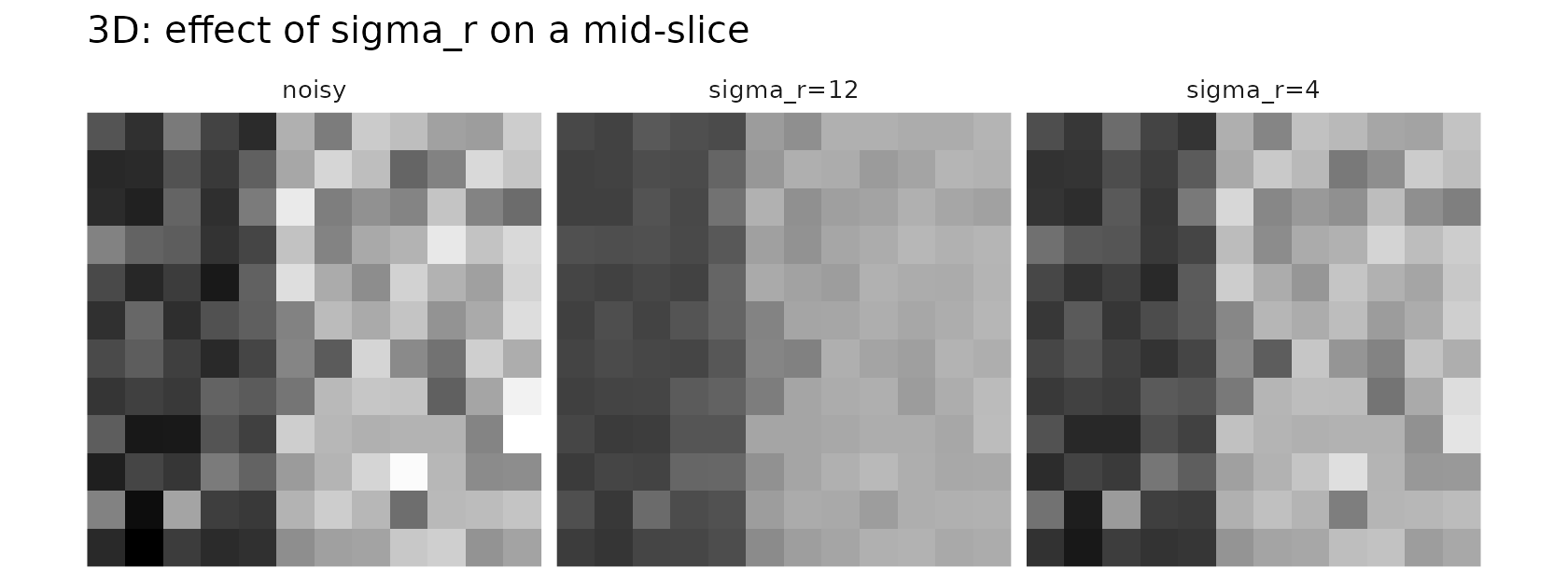

The smaller sigma_r preserves edges more aggressively at the cost of less denoising across intensity transitions. If no guide is supplied, the filter reduces to a purely spatial Gaussian smoothing and sigma_r has no effect.

4D example with temporal coupling

d4 <- c(10, 10, 10, 16)
base <- array(100, dim = d4)
base[6:10, , , ] <- base[6:10, , , ] + 20
noisy4d <- base + array(rnorm(prod(d4), sd = 5), dim = d4)

out_spat_only <- bilat_lattice4d(noisy4d, sigma_sp = 2.0, sigma_t = 0.0, sigma_r = 10)
out_spat_temp <- bilat_lattice4d(noisy4d, sigma_sp = 2.0, sigma_t = 0.6, sigma_r = 10)

c(var_spat_only = var(as.vector(out_spat_only)),
  var_spat_temp = var(as.vector(out_spat_temp)))
#> var_spat_only var_spat_temp 
#>      60.64485      60.76268

# visualize a central slice of a central frame
zmid <- ceiling(d4[3]/2); tmid <- ceiling(d4[4]/2)
viz4 <- rbind(
  slice_df4d(noisy4d, zmid, tmid, "noisy"),
  slice_df4d(out_spat_only, zmid, tmid, "sigma_t=0.0"),
  slice_df4d(out_spat_temp, zmid, tmid, "sigma_t=0.6")
)
ggplot(viz4, aes(x, y, fill = val)) +
  geom_raster() +
  coord_equal() +
  scale_x_continuous(expand = c(0,0), breaks = NULL) +
  scale_y_reverse(expand = c(0,0), breaks = NULL) +
  scale_fill_gradient(low = "black", high = "white") +
  facet_wrap(~method, nrow = 1) +
  guides(fill = "none") +
  theme_minimal(base_size = 10) +
  theme(axis.title = element_blank(), axis.text = element_blank(), panel.grid = element_blank()) +
  labs(title = "4D: temporal coupling on a mid-slice/frame")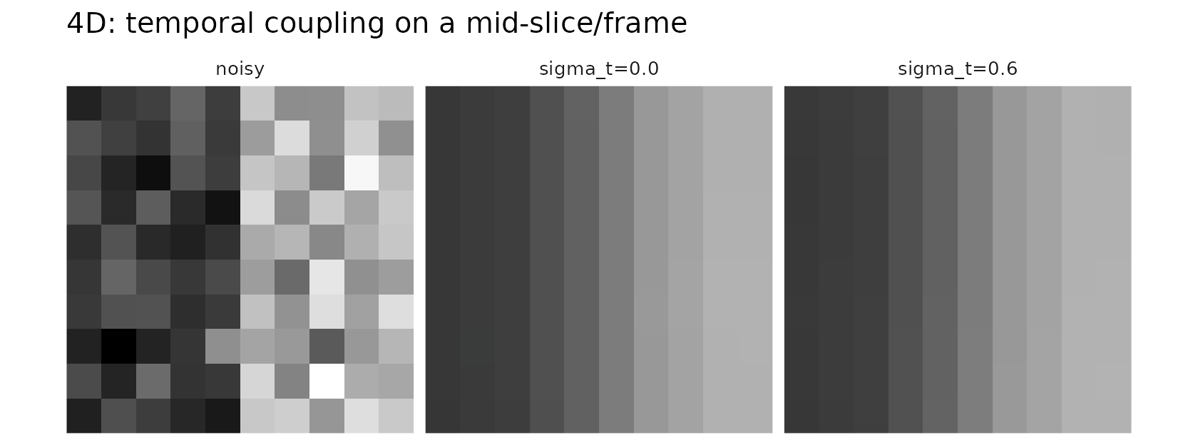

Increasing sigma_t introduces gentle temporal smoothing that can improve SNR if the signal is temporally coherent.

Design‑aware features

When you have a regressor (for example, an expected response over time), passing it as design adds a feature that keeps frames with similar design values closer in the lattice. This helps denoising without blurring across task‑related changes.

design <- sin(seq(0, 2*pi, length.out = d4[4]))
out_design <- bilat_lattice4d(noisy4d, sigma_sp = 2.0, sigma_t = 0.4, sigma_r = 10,
                              design = design, sigma_d = 1.0)
all.equal(dim(out_design), d4)
#> [1] TRUE

Practical tips

Start with sigma_sp around 2–3 voxels and sigma_r comparable to the noise scale. Add a small sigma_t (0.3–0.8) for 4D data. Use a higher sigma_r if you want stronger denoising with some edge rounding, and a lower one if preserving boundaries is critical.

fmrismooth authors