Edge-Preserving Guided Filtering (3D/4D)

fmrismooth authors

2025-08-28

Guided filtering is a fast, edge‑preserving smoother. Unlike bilateral filtering, it assumes a local linear model between the output and a guide image within each window. The regularization parameter prevents overfitting across noisy regions and avoids edge leakage.

This vignette shows how to use the 3D and 4D guided filters and how to choose their parameters.

Spatial guided filtering (3D)

The 3D variant processes one volume using a sliding window. The window radius controls spatial scale; the regularization eps sets how “rigid” the fit is to the guide: small values track edges more closely, larger values behave more like an averaging filter.

d3 <- c(10, 10, 10)
vol <- array(100, dim = d3)
vol[6:10, , ] <- vol[6:10, , ] + 20
noisy <- vol + array(rnorm(prod(d3), sd = 6), dim = d3)

gf_smooth <- guided_filter3d(noisy, radius = 2L, eps = 0.5^2)
gf_rigid  <- guided_filter3d(noisy, radius = 2L, eps = 1.5^2)

c(var_noisy = var(as.vector(noisy)),
  var_smooth = var(as.vector(gf_smooth)),
  var_rigid  = var(as.vector(gf_rigid)))
#>  var_noisy var_smooth  var_rigid 
#>   137.3983   136.9045   133.1892

zmid <- ceiling(d3[3]/2)
viz3 <- rbind(
  slice_df3d(noisy, zmid, "noisy"),
  slice_df3d(gf_smooth, zmid, "eps=0.25"),
  slice_df3d(gf_rigid, zmid, "eps=2.25")
)
ggplot(viz3, aes(x, y, fill = val)) + geom_raster() + coord_fixed() + scale_y_reverse() +
  scale_fill_gradient(low = "black", high = "white") + facet_wrap(~method) + theme_minimal(base_size = 10) +
  labs(title = "3D guided filter: mid-slice", x = NULL, y = NULL, fill = "intensity")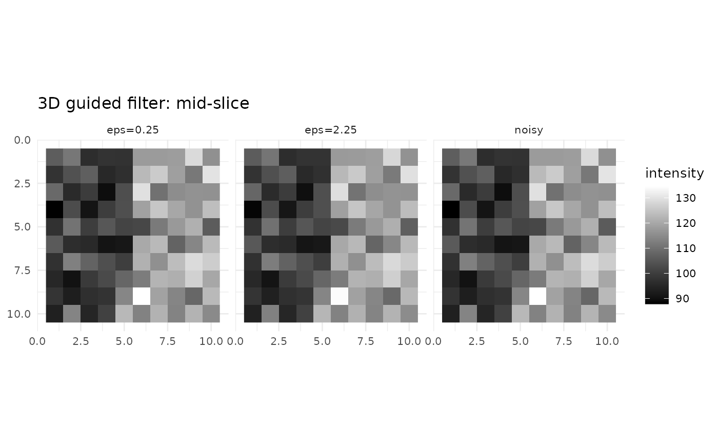

Using the input itself as the guide is common. You can also pass an external guide, for example a T1 anatomical, to steer the filter across low‑contrast fMRI regions.

Spatiotemporal guided filtering (4D)

The 4D variant applies the spatial guided filter to each frame, then an optional temporal guided step per voxel. The temporal radius sets how many frames on either side to include; eps_t plays the same role as in space. Motion‑aware temporal weights can down‑weight transitions between frames with large motion changes.

d4 <- c(8, 8, 8, 14)
x <- array(100, dim = d4) + array(rnorm(prod(d4), sd = 5), dim = d4)

out_no_temp <- guided_filter4d(x, radius_sp = 2L, eps_sp = 0.6^2, radius_t = 0L)
out_temp    <- guided_filter4d(x, radius_sp = 2L, eps_sp = 0.6^2, radius_t = 1L, eps_t = 0.3^2)

c(var_no_temp = var(as.vector(out_no_temp)),
  var_temp    = var(as.vector(out_temp)))
#> var_no_temp    var_temp 
#>    25.00629    24.83296

zmid <- ceiling(d4[3]/2); tmid <- ceiling(d4[4]/2)
viz4 <- rbind(
  slice_df4d(x, zmid, tmid, "noisy"),
  slice_df4d(out_no_temp, zmid, tmid, "radius_t=0"),
  slice_df4d(out_temp, zmid, tmid, "radius_t=1")
)
ggplot(viz4, aes(x, y, fill = val)) + geom_raster() + coord_fixed() + scale_y_reverse() +
  scale_fill_gradient(low = "black", high = "white") + facet_wrap(~method) + theme_minimal(base_size = 10) +
  labs(title = "4D guided filter: mid-slice/frame", x = NULL, y = NULL, fill = "intensity")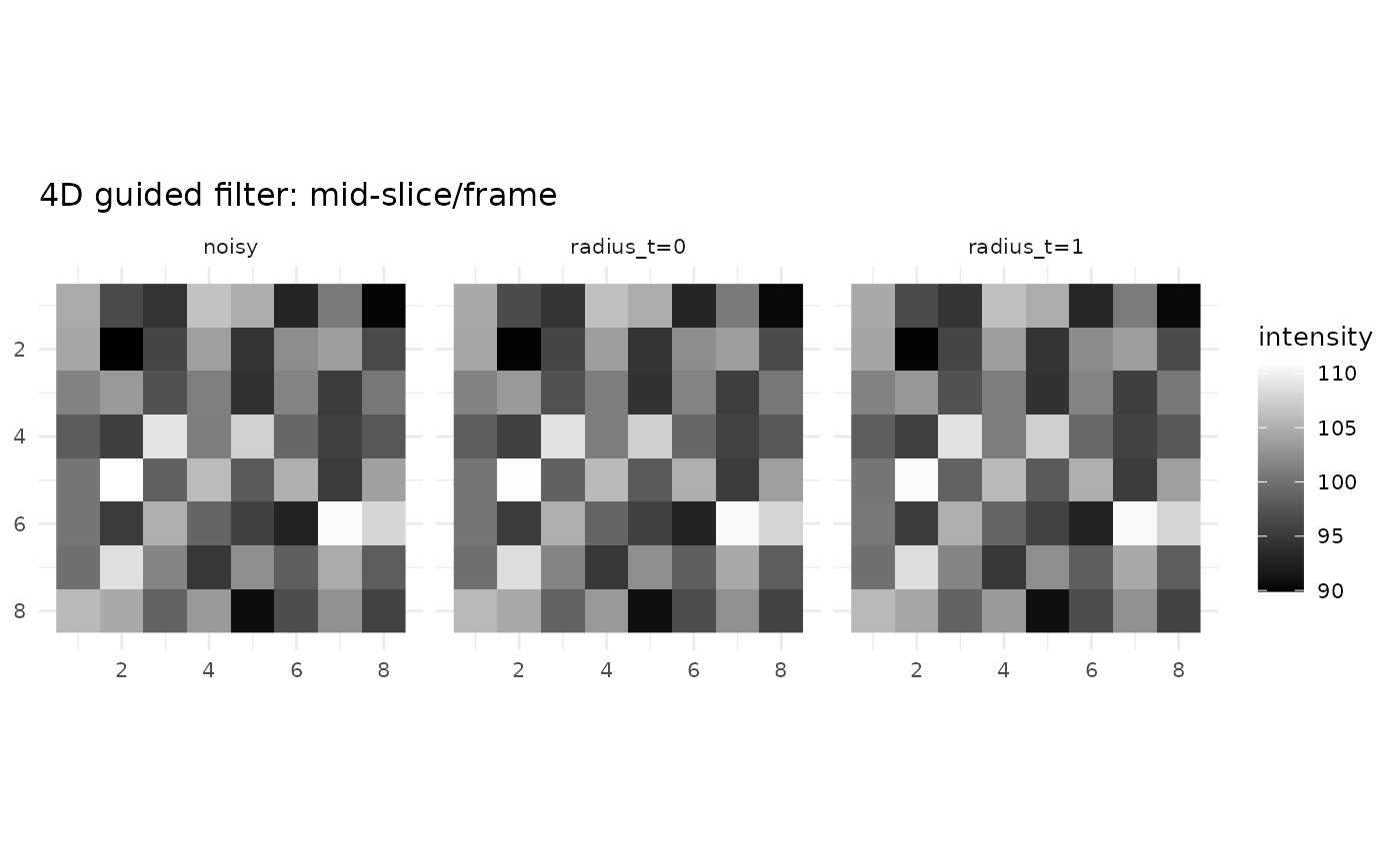

When you have per‑frame motion parameters, supply them as motion_params; the filter will dampen temporal averaging across high‑motion transitions.

Choosing parameters

Start with radius = 2–3 voxels and eps near the noise variance. For 4D, a temporal radius of 1 with a modest eps_t often helps without washing out transients. If edges look washed out, reduce eps; if banding or over‑fitting appears, increase it.