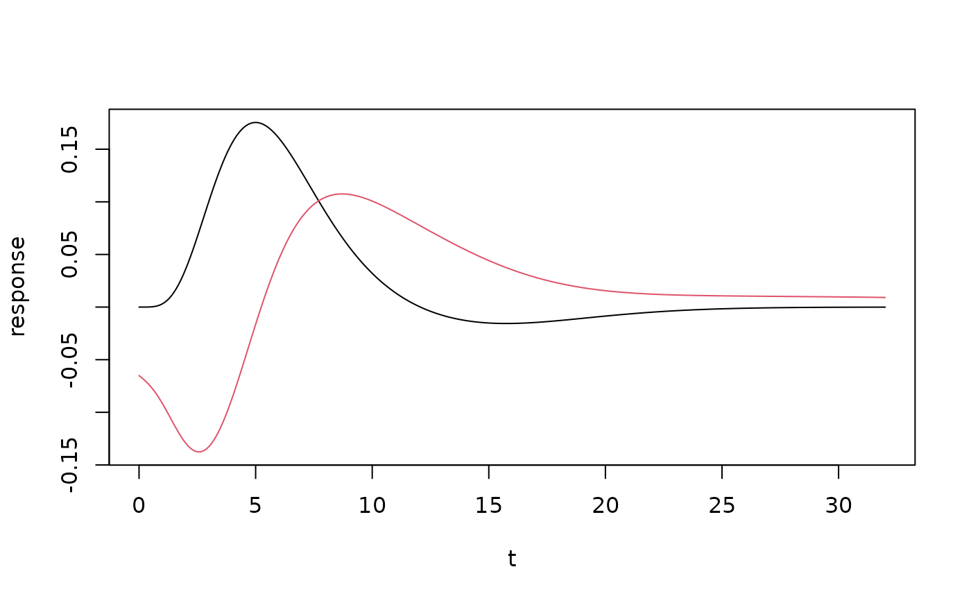
The Hilbert transform of the SPM canonical HRF ([hrf_spmg1()]) on `[0, span]`, made orthogonal to the canonical HRF and scaled to the same L2 norm. Together the two functions form a quadrature pair: a small shift of the response in time acts, to a good approximation, as a rotation of the two coefficients, so their length carries amplitude and their angle carries latency. The temporal derivative in [HRF_SPMG2] plays the same role but only for shifts of about a second.
Arguments
- t
A vector of time points.
- P1
The first exponent parameter (default: 5).
- P2
The second exponent parameter (default: 15). The undershoot is
t^P2 * exp(-t) / (6 * factorial(P2)), one sixth of a gamma density with shapeP2 + 1and unit rate.- A1
Amplitude scaling factor for the positive gamma function component; normally fixed at 1/120
- span
Length in seconds of the window on which the function is defined (default 32). It is zero outside `[0, span]`.
Details
The function is tabulated once per parameter set on a 0.01 s grid (the Hilbert transform is computed with a zero-padded FFT) and interpolated linearly. Unlike the canonical HRF, the Hilbert transform of a causal function is not causal, so the quadrature partner does not start at zero: restricted to `[0, span]` it begins at about -0.37 of the canonical peak. Treat it as a companion regressor for estimating latency, not as a response shape.
References
Saad, Z. S., Ropella, K. M., Cox, R. W., & DeYoe, E. A. (2001). Analysis and use of FMRI response delays. *Human Brain Mapping*, 13(2), 74-93. doi:10.1002/hbm.1026
See also
[HRF_SPMGQ], [amplitude_latency()]
Other hrf_functions:
hrf_basis_lwu(),
hrf_boxcar(),
hrf_bspline(),
hrf_gamma(),
hrf_gaussian(),
hrf_inv_logit(),
hrf_lwu(),
hrf_mexhat(),
hrf_sine(),
hrf_spmg1(),
hrf_time(),
hrf_weighted()