Principal component analysis starts with centering: subtract each
column’s mean before finding directions of maximum variance. For a
sparse matrix, that one subtraction is the problem.
A - 1 %*% t(col_means) fills in every zero with a small
nonzero number, so the matrix that started sparse becomes dense before
you’ve computed a single eigenvector.
eigencore solves the centered (and optionally scaled) problem as an operator, so the subtraction never happens as a stored matrix. This vignette builds one sparse dataset, centers and scales it, and computes a certified partial SVD without ever forming the dense copy.
Build a sparse dataset with a low-rank signal
Simulate the kind of matrix behind collaborative filtering and topic models: sparse interaction counts between 2,000 users and 500 items, built from five latent factors so a handful of singular vectors should recover most of the structure.
set.seed(1)
m <- 2000L; n <- 500L; k_true <- 5L
U <- qr.Q(qr(matrix(rnorm(m * k_true), m, k_true)))
V <- qr.Q(qr(matrix(rnorm(n * k_true), n, k_true)))
signal <- U %*% diag(seq(8, 4, length.out = k_true)) %*% t(V)
Only 4% of user-item pairs are observed, and the observations are noisy:
mask  <- rsparsematrix(m, n, density = 0.04)
noise <- rsparsematrix(m, n, density = 0.01, rand.x = function(k) rnorm(k, sd = 0.05))
A <- as((signal * (mask != 0)) + noise, "dgCMatrix")
dim(A)
#> [1] 2000  500
At 2,000 x 500 this is a small matrix, but the storage gap is already visible: a dense copy would need 7.6 MB, while the sparse representation needs 0.57 MB — about 13 times less.
Center without densifying
center() wraps A in an operator that
subtracts column means on the fly, computing the means directly from the
sparse matrix rather than requiring you to supply them.
Ac <- center(A, columns = TRUE)
Ac
#> <eigencore operator>
#>   name: center(sparse_csc_matrix)
#>   dim: 2000 x 500
#>   dtype: double
#>   structure: general
Pass the centered operator straight to svd_partial(),
exactly as you would the original matrix.
fit <- svd_partial(Ac, rank = 5, target = largest())
fit
#> Partial SVD
#>   requested rank: 5
#>   converged rank: 5
#>   method: native matrix-free Golub-Kahan callback cycle + native Ritz extraction (callback boundary)
#>   target: largest
#>   max residual: 5.968391e-11
#>   max backward error: 1.267432e-10
#>   max orthogonality loss: 1.332268e-15
#>   norm bound: two_norm_lower_bound
#>   scale estimated: FALSE
#>   certificate: passed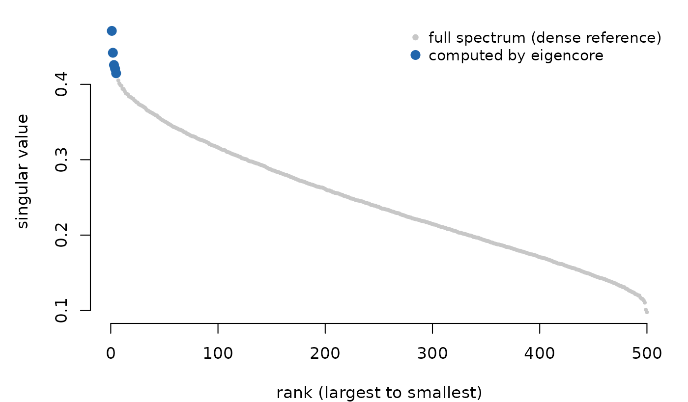
The five largest singular values of the centered matrix (blue) against the full singular spectrum (grey).
The five leading singular values separate cleanly from the rest of the spectrum — exactly what you’d expect from data built around five latent factors.
Read the certificate on a composed operator
The centered operator is never formed, yet its certificate can still pass:
fit$certificate$passed
#> [1] TRUE
fit$certificate$max_backward_error
#> [1] 1.267432e-10
fit$certificate$norm_bound_type
#> [1] "two_norm_lower_bound"
fit$certificate$scale_is_estimate
#> [1] FALSE
The backward error divides each residual by a lower bound on
||A_c||_2 (two_norm_lower_bound): here the
largest ||A_c v|| / ||v|| over the computed singular
vectors, which for the leading triplets is essentially the exact norm. A
lower bound in the denominator can only over-state the backward error,
so the check is never optimistic, and it needs no second pass over the
data. The same holds for operators without any norm metadata (a
double-centered matrix or a hand-written callback);
vignette("certificates") covers the rule in detail.
Does it match what you’d get by densifying?
The whole point of center() is that it should be
numerically indistinguishable from centering the dense matrix directly.
Check it:
The two agree to machine precision. dense_centered above
was built only to draw the comparison plot and run this check — the
eigencore computation itself never materialized it.
Scale columns too
A common next step in PCA preprocessing is scaling each column to
unit variance, turning a covariance-matrix PCA into a correlation-matrix
one. Compute the column variances from the sparse matrix and pass them
to scale_cols(), composed with the centering operator you
already have:
col_var <- Matrix::colMeans(A^2) - Matrix::colMeans(A)^2
w <- 1 / sqrt(col_var + 1e-6)
Acs <- scale_cols(Ac, w)
fit_scaled <- svd_partial(Acs, rank = 5, target = largest())
fit_scaled$d
#> [1] 75.68299 71.50447 68.85755 66.99968 65.85421
fit_scaled$certificate$passed
#> [1] TRUE
fit_scaled$certificate$norm_bound_type
#> [1] "two_norm_lower_bound"
fit_scaled$certificate$scale_is_estimate
#> [1] FALSE
center() and scale_cols() compose freely
because both return the same eigencore_operator type that
every solver accepts — there’s no separate “scaled matrix” object to
keep track of. For this column-centered CSC composition, eigencore also
reuses the sparse column moments to compute the exact Frobenius norm
sum_j w_j^2 sum_i (A_ij - mean_j)^2, kept as diagnostic
metadata. The certificate itself scales by a lower bound on the 2-norm,
so the scaled solve passes even though the centered matrix itself is
never formed.
What did the planner actually do?
Every solve is preceded by a plan. Inspect it before the solve when method selection, densification, or fallback behavior matters:
plan <- plan_solver(svd_problem(Acs), rank = 5, target = largest())
plan$method
#> [1] "native prototype Golub-Kahan"
plan$reasons
#> [1] "target: largest"
#> [2] "rectangular SVD problem"
#> [3] "adjoint is available"
#> [4] "default avoids normal equations"
#> [5] "centered-plus-column-scaled CSC operator has a fused native block apply and direct native Golub-Kahan cycle without an R callback boundary"
Centering and scaling a CSC matrix fuse into a single native,
non-densifying construction. The planner routes that operator to a
direct native Golub-Kahan cycle: the C++ hot loop consumes the original
CSC slots, column means, and scale weights without an R callback
boundary. Inspect plan$controls$fused_centered_scaled_csc
and plan$controls$callback_boundary for the
machine-readable contract; the human-readable reasons state
the same boundary. plan_solver() takes the same
problem/rank/target arguments as the solve itself, so you can check the
route before paying for the computation.
When can the Gram matrix stay implicit?
An SVD route based on A^T A or A A^T does
not have to construct that Gram matrix. When the smaller side is too
large or poorly shaped for the bounded explicit-Gram path, eigencore can
apply the normal operator implicitly and run a restarted eigensolver on
that action.
Use a square slice of the same sparse dataset to make the distinction visible. Its shape offers no small explicit Gram matrix, but the operator and its adjoint are still available:
square_slice <- A[seq_len(96), seq_len(96)]
implicit_plan <- plan_solver(
  svd_problem(square_slice),
  rank = 4,
  target = largest()
)
implicit_fit <- solve(implicit_plan)

data.frame(
  planned = implicit_fit$planned_method,
  actual = implicit_fit$actual_method,
  fallback = implicit_fit$fallback_used,
  certified = certificate(implicit_fit)$passed
)
#>                                                      planned
#> 1 native certified implicit Gram SVD (thick-restart Lanczos)
#>                                                       actual fallback certified
#> 1 native certified implicit Gram SVD (thick-restart Lanczos)    FALSE      TRUE
The plan says both what is avoided and what remains certified: the
Gram matrix is not materialized, while the returned singular triplets
are checked in the original coordinates. This is a routing decision, not
a recommendation to form normal equations yourself; call
svd_partial() or execute the inspected plan and let the
certificate judge the returned triplets.
Going fully matrix-free
Sometimes there’s no matrix at all — just a function that knows how
to apply A and its adjoint. linear_operator()
wraps arbitrary callbacks the same way center() wraps a
sparse matrix.
op <- linear_operator(
  dim = dim(A),
  apply = function(X, alpha = 1, beta = 0, Y = NULL) {
    # Sparse %*% dense returns an S4 dgeMatrix; as.matrix() keeps the
    # callback's return type consistent with what the native solver expects.
    Z <- alpha * as.matrix(A %*% X)
    if (is.null(Y) || beta == 0) Z else Z + beta * Y
  },
  apply_adjoint = function(X, alpha = 1, beta = 0, Y = NULL) {
    Z <- alpha * as.matrix(crossprod(A, X))
    if (is.null(Y) || beta == 0) Z else Z + beta * Y
  },
  name = "matrix-free A"
)
fit_mf <- svd_partial(op, rank = 5, target = largest())
fit_mf$certificate$norm_bound_type
#> [1] "two_norm_lower_bound"
Even without any norm metadata the certificate scales by a 2-norm
lower bound taken from the computed vectors, so it can pass. Norm
metadata is still useful: an exact Frobenius norm gives a cheap
structural floor (||A||_F / sqrt(min(m, n))) before any
vector is computed, and metadata$two_norm, when you know
it, makes the scale exact:
op_hinted <- linear_operator(
  dim = dim(A),
  apply = op$apply,
  apply_adjoint = op$apply_adjoint,
  name = "matrix-free A (exact norm)",
  metadata = list(frobenius_norm = norm(A, type = "F"))
)
fit_hinted <- svd_partial(op_hinted, rank = 5, target = largest())
fit_hinted$certificate$norm_bound_type
#> [1] "two_norm_lower_bound"
fit_hinted$certificate$norm_source
#> [1] "applied_vectors"
fit_hinted$certificate$passed
#> [1] TRUE
Whether you reach for center()/scale_cols()
or hand-write a linear_operator(), the certificate always
tells you which kind of evidence backed the result.
Why this matters at scale
The 2,000 x 500 example above keeps this vignette fast to build, but the memory argument only gets sharper as the matrix grows. A production recommender with 5 million users and 200,000 items would need roughly 8 TB to store as a dense matrix; the sparse representation, at typical interaction densities, fits in a few gigabytes. Densifying to center it would defeat the entire point of using a sparse format.
Where to go next
-
vignette("certificates")— the deep dive onpassed,norm_bound_type, and what to do when a certificate fails. -
vignette("eigencore")— the general get-started workflow: operators, problems, plans, and solves for both eigenproblems and SVD. -
vignette("generalized-eigenproblems")— problems of the formA v = lambda B v, including whitened and metric-weighted variants. -
?linear_operatorand?composedocument the full operator algebra, includingcrossprod_operator()for buildingA^* Awhen an eigenproblem is a more natural fit than an SVD.