Get started with eigencore

eigencore turns spectral computation into a five-step workflow:

1. Build an operator describing the action of A.
2. Describe the problem (eigen or SVD; metric B; spectral target).
3. Plan a solver and inspect what it will run.
4. Solve.
5. Inspect the certificate — the numerical evidence that the result is trustworthy.

This vignette walks through the workflow on three problem classes: a standard Hermitian eigenproblem, a generalized SPD eigenproblem with a metric B, and a partial SVD. It also shows the RSpectra-compatible shim for users migrating from existing code.

For the V2 CRAN release, planner labels are part of the contract: promoted paths are native and benchmark-backed in their documented regimes, while reference, prototype, oracle, and diagnostic paths remain clearly labelled.

library(eigencore)

1. Standard Hermitian eigenproblem

Build a small symmetric matrix and ask for the five largest eigenvalues.

set.seed(1)
n <- 200
A <- crossprod(matrix(rnorm(n * n), n, n)) / n + diag(n)

eigencore wraps the matrix in a block-native operator the moment you hand it to a problem constructor. You can do this explicitly:

Aop <- as_operator(A)
Aop
#> <eigencore operator>
#>   name: dense_matrix 
#>   dim: 200 x 200 
#>   dtype: double 
#>   structure: hermitian

The operator carries dimensions, structure tags, and a flag indicating whether the underlying storage has a native kernel (in this case dense double — yes).

Build the problem and inspect the plan

P    <- eigen_problem(A, structure = hermitian(), target = largest())
plan <- plan_solver(P, k = 5)
plan
#> eigencore solver plan
#>   problem: eigen 
#>   requested: 5 
#>   target: largest 
#>   method: native scalar thick-restart Hermitian Lanczos 
#>   reasons:
#>    - structure: hermitian 
#>    - target: largest 
#>    - standard eigenproblem 
#>    - built-in dense operator has native block apply 
#>   controls:
#>    - block : 1 
#>    - max_subspace : 35 
#>    - max_restarts : 100 
#>    - reorthogonalize : TRUE 
#>   fallback: dense oracle prototype if unsupported

The plan tells you exactly which kernel will be invoked. There is no silent dispatch.

Solve and read the certificate

fit <- solve(P, k = 5)
fit
#> Partial eigen decomposition
#>   requested: 5 
#>   converged: 5 
#>   method: native scalar thick-restart Hermitian Lanczos 
#>   target: largest 
#>   restart:thick_restart(in_native_loop)
#>   locked: 5 
#>   max residual: 1.67046e-07 
#>   max backward error: 4.546939e-09 
#>   max orthogonality loss: 1.776357e-15 
#>   norm bound: frobenius_exact+identity_exact 
#>   scale estimated: FALSE 
#>   certificate: passed

fit$certificate
#> eigencore certificate
#>   passed: TRUE 
#>   tolerance: 1e-08 
#>   type: residual_backward_error 
#>   norm bound: frobenius_exact+identity_exact 
#>   scale estimated: FALSE 
#>   max residual: 1.67046e-07 
#>   max backward error: 4.546939e-09 
#>   max orthogonality loss: 1.776357e-15 
#>   orthogonality tolerance: 1.490116e-08 
#>   orthogonality required: TRUE

A passing certificate means: every requested pair has

• residual ||A v - lambda v|| / s below tol, where s is the labeled norm bound (here frobenius_exact),
• backward error below tol,
• inter-vector orthogonality loss below the orthogonality tolerance.

The certificate is not one number — it is one verdict per returned pair. Plot the per-pair backward error and the tolerance becomes a line you can see every pair clearing.

Per-pair backward error for the five returned eigenpairs. Every pair sits well below the dashed tolerance line, so the overall certificate passes.

If any pair were above the line, the certificate’s failed_indices slot would name it. Here the worst pair clears the tolerance by orders of magnitude.

fit$values
#> [1] 5.010576 4.769169 4.700866 4.566055 4.504502

These five values are a certified slice of a 200-dimensional spectrum. Plotting them against the full dense spectrum shows exactly which part of the problem you paid to compute.

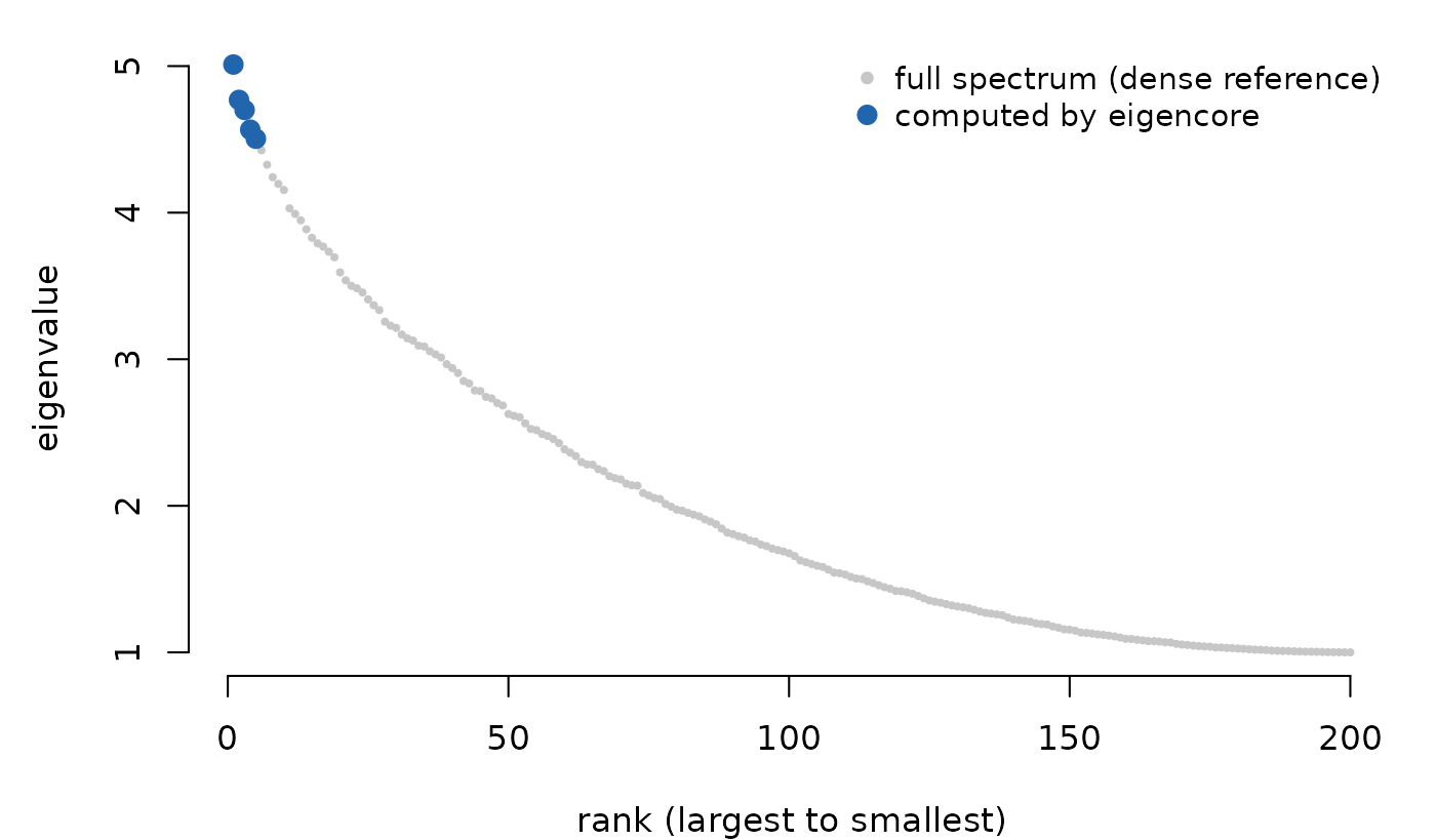
The five largest eigenvalues (blue) located within the full spectrum of A (grey). eigencore computes only the requested slice, then certifies it.

With n = 200 we asked for 5 of 200 pairs. In a production problem with n = 1e6, computing the full spectrum is impossible — the partial result is the only result, which is exactly why a certificate matters.

2. Generalized SPD eigenproblem (A v = lambda B v)

Pass a metric B to eigen_problem() (or to eig_partial() via the B argument).

B <- diag(seq(1, 5, length.out = n))
fit_gen <- eig_partial(A, k = 5, target = largest(), B = B,
                       method = lobpcg(maxit = 200))
fit_gen
#> Partial eigen decomposition
#>   requested: 5 
#>   converged: 5 
#>   method: native generalized SPD LOBPCG (B-orthogonal, residual certified) 
#>   target: largest 
#>   restart: lobpcg 
#>   locked: 5 
#>   max residual: 9.243565e-09 
#>   max backward error: 7.47322e-11 
#>   max orthogonality loss: 1.44329e-15 
#>   norm bound: frobenius_exact+frobenius_exact 
#>   scale estimated: FALSE 
#>   certificate: passed

The certificate’s residual is ||A v - lambda B v|| / (||A|| + |lambda| ||B||), and orthogonality is measured in the B-inner product where appropriate. The norm_bound_type now reports a bound for both A and B.

3. Partial SVD

For rectangular problems use svd_partial():

M <- matrix(rnorm(400 * 50), 400, 50)
svd_fit <- svd_partial(M, rank = 5, target = largest())
svd_fit
#> Partial SVD
#>   requested rank: 5 
#>   converged rank: 5 
#>   method: native certified Gram SVD special case 
#>   target: largest 
#>   max residual: 1.359395e-15 
#>   max backward error: 9.520164e-18 
#>   max orthogonality loss: 5.689893e-16 
#>   norm bound: frobenius_exact 
#>   scale estimated: FALSE 
#>   certificate: passed

The same mental model applies to singular values: you compute the leading few and leave the tail untouched.

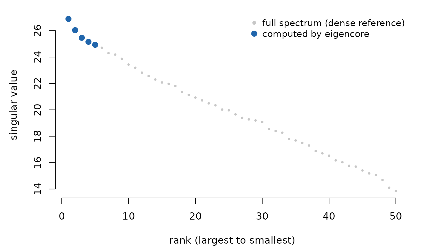
The five leading singular values (blue) computed by eigencore, shown against the full singular-value spectrum of M (grey).

The reported method identifies the path — for very small or near-square problems eigencore may use a dense LAPACK SVD fallback rather than running its iterative Golub–Kahan kernel. Either way the certificate covers both ||A v - sigma u|| and ||A^T u - sigma v||.

4. RSpectra-compatible workflow

If your existing code uses RSpectra::eigs_sym(), you can call eigencore in the same shape — the return list extends RSpectra’s by adding certificate and diagnostics:

res <- eigs_sym(A, k = 5, which = "LA")
str(res, max.level = 1)
#> List of 7
#>  $ values     : num [1:5] 5.01 4.77 4.7 4.57 4.5
#>  $ vectors    : num [1:200, 1:5] 0.0227 0.0103 0.0923 -0.1479 -0.0414 ...
#>  $ nconv      : int 5
#>  $ niter      : int 60
#>  $ nops       : int 62
#>  $ certificate:List of 18
#>   ..- attr(*, "class")= chr "eigencore_certificate"
#>  $ diagnostics:List of 15

res$certificate
#> eigencore certificate
#>   passed: TRUE 
#>   tolerance: 1e-08 
#>   type: residual_backward_error 
#>   norm bound: frobenius_exact+identity_exact 
#>   scale estimated: FALSE 
#>   max residual: 2.074433e-09 
#>   max backward error: 5.646539e-11 
#>   max orthogonality loss: 8.881784e-16 
#>   orthogonality tolerance: 1.490116e-08 
#>   orthogonality required: TRUE

eigs(), eigs_sym(), and svds() accept the same which codes as RSpectra — "LM", "SM", "LA", "SA", "LR", "SR", "LI", "SI", and "BE".

Where to go next

• vignette("certificates") is the deep dive on reading the numerical evidence — what each field means and what to do when a check fails.
• Run help(package = "eigencore") to browse the installed help index.
• ?certificate documents the certificate fields in detail.
• ?plan_solver explains how operator structure, target, and method combine to choose a kernel.
• linear_operator() lets you wrap a matrix-free apply callback as a first-class operator; eigencore’s planner will warn when an R-level callback is being driven from a block-native solver hot loop, so you can decide whether to invest in a native operator implementation.