Generalized eigenvalue problems with eigencore • eigencore

A generalized eigenvalue problem asks for nonzero vectors $x$ and scalars $\lambda$ satisfying

$A x = \lambda B x.$

This form shows up whenever a problem needs a metric other than the standard inner product: whitened PCA and canonical correlation analysis weight by a covariance matrix, linear discriminant analysis weights by a within-class scatter matrix, and normalized graph Laplacians weight by a degree matrix. In each case B is not incidental — solving the plain eigenproblem A x = lambda x and ignoring B gives you the wrong answer.

The second matrix $B$ may define a positive-definite metric, or it may be part of a more general matrix pencil. eigencore supports both cases, along with partial solves when you need only a few eigenpairs and QZ decompositions when you need the full structure of a dense pencil.

Start with a positive-definite metric

When A is symmetric (or Hermitian) and B is symmetric positive definite, pass B directly to eig_full(). The returned vectors are normalized in the $B$ metric.

A <- diag(c(2, 8, 18))
B <- diag(c(1, 2, 3))

fit <- eig_full(A, B = B)
values(fit)
#> [1] 2 4 6
certificate(fit)$passed
#> [1] TRUE

Here the generalized eigenvalues are 2, 4, and 6: each diagonal entry of A is divided by the corresponding entry of B.

Compute only part of the spectrum

Use eig_partial() when you need only a few eigenpairs. A target such as smallest() states which part of the spectrum to compute. Scale the same idea up to a diagonal metric problem with 150 pairs, and ask for the 5 smallest:

n <- 150
A_wide <- diag(seq(1, 150, length.out = n))
B_wide <- diag(seq(1, 2, length.out = n))

part <- eig_partial(A_wide, B = B_wide, k = 5, target = smallest())
sort(Re(values(part)))
#> [1] 1.000000 1.986667 2.960265 3.921053 4.869281
part$method
#> [1] "native dense generalized SPD LAPACK fallback"
certificate(part)$passed
#> [1] TRUE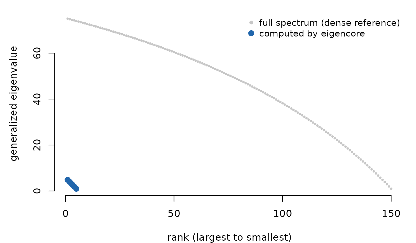

Scatter plot of 150 generalized eigenvalues sorted descending in grey, with the five smallest highlighted in blue at the bottom-right.

The five smallest generalized eigenvalues (blue) against the full 150-pair spectrum of the pencil (A, B) (grey).

With n = 150 this computed 5 of 150 pairs. A whitened-PCA or normalized-Laplacian problem built from real data routinely has n in the tens or hundreds of thousands, where a full generalized eigendecomposition is not practical — the partial slice, certified, is the only result you can afford.

The main choice is the structure of the problem and how much of its spectrum you need:

Problem	Function
Symmetric/Hermitian `A` with positive-definite `B`, full spectrum	`eig_full(A, B = B)`
Symmetric/Hermitian `A` with positive-definite `B`, partial spectrum	`eig_partial(A, B = B, k = ...)`
Dense general pencil	`eig_full(A, B = B, structure = general())`
Dense generalized Schur decomposition	`generalized_schur(A, B)`
Two dense maps with the same column domain	`generalized_svd(A, B)`

Handle a dense general pencil

Use structure = general() when B is indefinite, singular, nonsymmetric, or when the pair does not satisfy the symmetric/Hermitian positive-definite contract. This path represents eigenvalues by homogeneous coordinates $(\alpha, \beta)$ , where a finite eigenvalue is $\alpha / \beta$ .

A_general <- matrix(c(1, 4, 2, 3), 2, 2)
B_general <- matrix(c(2, 1, 0, -1), 2, 2)

pencil <- eig_full(A_general, B = B_general, structure = general())
coordinates <- alpha_beta(pencil)
values(pencil)
#> [1] -0.75+1.391941i -0.75-1.391941i
coordinates$classification
#> [1] "finite" "finite"
coordinates$classification_policy[c("policy", "tolerance")]
#> $policy
#> [1] "pencil_norm_scaled"
#> 
#> $tolerance
#> [1] 1.490116e-08
certificate(pencil)$passed
#> [1] TRUE

For a general pencil, right vectors satisfy A v = lambda B v, while left vectors satisfy the adjoint equation. Inspect both certificates when the left basis matters to sensitivity or biorthogonal projections:

W <- left_vectors(pencil)
c(
  right_certificate = certificate(pencil)$passed,
  left_certificate = pencil$left_certificate$passed
)
#> right_certificate  left_certificate 
#>              TRUE              TRUE

The classification policy is part of the result because “finite” depends on the numerical contract used to interpret (alpha, beta). Do not replace it with an unrecorded comparison such as abs(beta) < 1e-8.

Homogeneous coordinates are especially useful when B is singular. eigencore classifies finite, infinite, and undefined eigenvalues instead of forcing every pair into an ordinary numeric ratio.

singular <- eig_full(
  diag(c(2, 3, 0)),
  B = diag(c(1, 0, 0)),
  structure = general()
)

alpha_beta(singular)$classification
#> [1] "finite"    "infinite"  "undefined"
certificate(singular)$failed_indices
#> [1] 2 3

Use QZ when you need the Schur form

generalized_schur() computes a dense generalized Schur, or QZ, decomposition. Use values() for the finite ratios and alpha_beta() when you need the homogeneous coordinates or finite/infinite classification.

qz <- generalized_schur(A_general, B_general)
values(qz)
#> [1] -0.75+1.391941i -0.75-1.391941i
alpha_beta(qz)$classification
#> [1] "finite" "finite"
qz$method
#> [1] "native dense generalized Schur QZ LAPACK full"

For pencils with singular B, sort = "finite" or sort = "infinite" moves the requested class to the leading part of the decomposition.

qz_singular <- generalized_schur(
  diag(c(2, 3, 0)),
  diag(c(1, 0, 0)),
  sort = "infinite"
)
alpha_beta(qz_singular)$classification
#> [1] "infinite"  "finite"    "undefined"

When do you need a generalized SVD instead?

A generalized eigenproblem compares two square operators through A x = lambda B x. A generalized SVD answers a different question: two possibly rectangular matrices act on the same column direction, and you want to compare the strength of those two actions. The matrices must have the same number of columns, but they may have different numbers of rows.

For diagonal maps, the generalized singular values are easy to anticipate: each value is the corresponding strength in A divided by the strength in B.

A_gsvd <- diag(c(3, 4, 5))
B_gsvd <- diag(c(4, 3, 2))
gsvd_fit <- generalized_svd(A_gsvd, B_gsvd, tol = 1e-10)
gsvd_coordinates <- alpha_beta(gsvd_fit)

data.frame(
  alpha = gsvd_coordinates$alpha,
  beta = gsvd_coordinates$beta,
  value = gsvd_coordinates$values,
  classification = gsvd_coordinates$classification
)
#>       alpha      beta    value classification
#> 1 0.6000000 0.8000000 0.750000         finite
#> 2 0.8000000 0.6000000 1.333333         finite
#> 3 0.9284767 0.3713907 2.500000         finite

Here alpha^2 + beta^2 = 1 for every pair. alpha / beta is finite whenever beta is positive, even when it is very small. The returned classification_policy records that structural rule separately from tol, which controls reconstruction and orthogonality certification.

Rank-deficient rectangular pairs can contain finite, infinite, and undefined structural positions at once:

A_rect <- matrix(
  c(1, 2, 3, 3, 2, 1, 4, 5, 6, 7, 8, 8),
  nrow = 2,
  byrow = TRUE
)
B_rect <- matrix(1:18, ncol = 6, byrow = TRUE)
gsvd_rect <- generalized_svd(A_rect, B_rect, tol = 1e-7)
rect_coordinates <- alpha_beta(gsvd_rect)

data.frame(
  value = rect_coordinates$values,
  classification = rect_coordinates$classification
)
#>   value classification
#> 1   Inf       infinite
#> 2   Inf       infinite
#> 3     0         finite
#> 4     0         finite
#> 5    NA      undefined
#> 6    NA      undefined

Inf means beta = 0 while alpha is nonzero. NA represents a trailing structural (0, 0) pair, not an accidentally missing computation. Keeping the full length-ncol(A) layout lets classifications, factor columns, and reconstruction metadata stay aligned. Use left_vectors(gsvd_fit) and right_vectors(gsvd_fit) for the two row-space factors; the shared column factor remains gsvd_fit$Q.

Keep sparse partial problems sparse

Sparse symmetric/Hermitian problems with a positive-definite metric use eig_partial(). Set allow_dense_fallback = "never" when preserving sparsity is a hard requirement.

A_sparse <- Diagonal(x = c(1, 4, 9, 16, 25, 36))
B_sparse <- Diagonal(x = c(1, 2, 3, 4, 5, 6))

sparse_fit <- eig_partial(
  A_sparse,
  B = B_sparse,
  k = 3,
  target = smallest(),
  method = lanczos(max_subspace = 6),
  allow_dense_fallback = "never"
)

values(sparse_fit)
#> [1] 1 2 3
sparse_fit$method
#> [1] "native transformed generalized SPD B-orthogonal Lanczos"
certificate(sparse_fit)$passed
#> [1] TRUE

Full-spectrum functions accept base dense matrices and reject sparse or operator inputs rather than silently converting them to dense storage.

A note for older code

The retired geigen package exposed related operations, but eigencore is not a namespace-compatible replacement. When maintaining older code, translate the mathematical operation: use eig_full() for a full generalized eigensolve, generalized_schur() for QZ, generalized_svd() for a GSVD, and alpha_beta() to inspect homogeneous coordinates.

Where to go next

vignette("sparse-pca") covers operators and non-densifying centering for the standard (non-generalized) eigenproblem and SVD.
For more on result validation, see vignette("certificates").
?generalized_svd documents the returned factors and reconstruction layout.