This vignette demonstrates how to interpret the components extracted by DKGE, shows techniques for rotating them to achieve specific interpretations when needed, and explains how to project new data into the fitted component space.
Example Fit
library(dkge)
S <- 4; q <- 5; P <- 18; T <- 70
betas <- replicate(S, matrix(rnorm(q * P), q, P), simplify = FALSE)
designs <- replicate(S, {
  X <- matrix(rnorm(T * q), T, q)
  qr.Q(qr(X))
}, simplify = FALSE)
subjects <- lapply(seq_len(S), function(s) dkge_subject(betas[[s]], designs[[s]], id = paste0("sub", s)))
bundle <- dkge_data(subjects)
fit <- dkge(bundle, K = diag(q), rank = 3)
By default dkge() pools the whitened subject covariances
and diagonalises the result.
To enforce a joint diagonalisation across subjects—often yielding more
stable components— set solver = "jd" (and optionally pass
jd_control = dkge_jd_control(...) to tweak the
optimiser):
fit_jd <- dkge(bundle,
               K = diag(q),
               rank = 3,
               solver = "jd",
               jd_control = dkge_jd_control(maxit = 200, tol = 1e-8))
Both solvers return the same object structure (fit$U,
fit$Chat, projections, etc.), so the subsequent workflow in
this vignette applies unchanged regardless of the solver choice.
Inspect Loadings and Scores
round(fit$U, 3)         # effect-space loadings
#>        [,1]   [,2]   [,3]
#> [1,]  0.143  0.950 -0.072
#> [2,] -0.123  0.016  0.018
#> [3,] -0.281  0.290 -0.132
#> [4,] -0.120 -0.098 -0.977
#> [5,]  0.933 -0.068 -0.152
lapply(fit$Btil, function(Bts) round(Bts[, 1:3, drop = FALSE], 2))[1]
#> [[1]]
#>         cluster_1 cluster_2 cluster_3
#> effect1      1.96      2.58     -3.34
#> effect2      0.94      1.07      0.94
#> effect3     -0.22     -0.25      1.66
#> effect4     -0.43     -2.45      0.59
#> effect5      2.32     -2.24     -6.55
The columns of fit$U represent the loadings for each
component in the effect space. These loadings define how the original
design effects combine to form the extracted components. The
Btil element stores the subject-specific beta matrices
after row-standardization, which ensures comparable scaling across
subjects. To obtain cluster scores for each component, these
standardized betas are multiplied with the corresponding columns of
fit$U.
Projecting Subjects into Component Space
subject_scores <- dkge_project_btil(fit, fit$Btil)
str(subject_scores, max.level = 1)
#> List of 4
#>  $ : num [1:18, 1:3] 2.438 -1.49 -7.243 -3.436 0.454 ...
#>   ..- attr(*, "dimnames")=List of 2
#>  $ : num [1:18, 1:3] 1.03 2.52 -2.46 -2.48 -1.41 ...
#>   ..- attr(*, "dimnames")=List of 2
#>  $ : num [1:18, 1:3] -0.781 1.226 1.925 -4.357 2.18 ...
#>   ..- attr(*, "dimnames")=List of 2
#>  $ : num [1:18, 1:3] 2.317 1.057 0.45 4.509 -0.595 ...
#>   ..- attr(*, "dimnames")=List of 2
Each subject score matrix has dimensions clusters × components, providing a complete mapping of how each brain cluster expresses each component. Computing average scores across subjects provides a useful summary that reveals the overall spatial patterns of component expression.
avg_scores <- Reduce("+", subject_scores) / length(subject_scores)
avg_df <- as.data.frame(avg_scores)
component_cols <- paste0("Component ", seq_len(ncol(avg_df)))
names(avg_df) <- component_cols
avg_df$Cluster <- seq_len(nrow(avg_df))
avg_long <- tidyr::pivot_longer(avg_df,
                                cols = component_cols,
                                names_to = "Component",
                                values_to = "Score")
#> Warning: Using an external vector in selections was deprecated in tidyselect 1.1.0.
#> ℹ Please use `all_of()` or `any_of()` instead.
#>   # Was:
#>   data %>% select(component_cols)
#>
#>   # Now:
#>   data %>% select(all_of(component_cols))
#>
#> See <https://tidyselect.r-lib.org/reference/faq-external-vector.html>.
#> This warning is displayed once per session.
#> Call `lifecycle::last_lifecycle_warnings()` to see where this warning was
#> generated.

ggplot(avg_long, aes(x = Cluster, y = Score, colour = Component)) +
  geom_line(linewidth = 1.1) +
  labs(title = "Average component scores", y = "Score") +
  scale_x_continuous(breaks = seq_len(nrow(avg_scores))) +
  theme(legend.position = "top")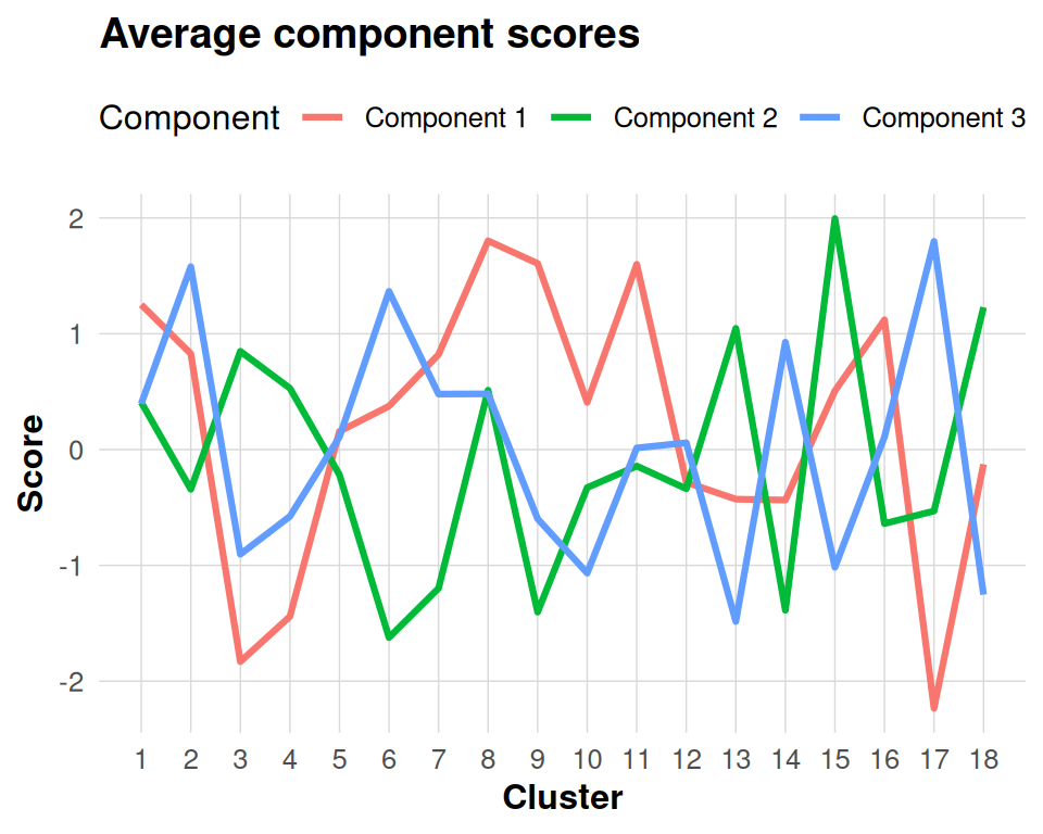
Rotating Components
The dkge_procrustes_K() function provides a principled
way to rotate components toward a target basis, such as canonical
contrasts or previously established loadings from prior studies. This
rotation preserves the mathematical properties of the solution by
staying within the design-kernel metric space.
# target basis: identity for first two effects
B_target <- diag(1, q)[, 1:2]
rot <- dkge_procrustes_K(fit$U[, 1:2], B_target, fit$K)
round(rot$R, 3)
#>       [,1]   [,2]
#> [1,] 0.146 -0.989
#> [2,] 0.989  0.146
The rotation matrix rot$R can then be applied by
multiplying it with the original loadings to obtain the aligned
components that are oriented toward the target basis.
Projecting New Data
new_beta <- matrix(rnorm(q * P), q, P)
projected <- dkge_project_clusters(fit, new_beta)
head(projected)
#>          [,1]    [,2]    [,3]
#> [1,] -0.08667  0.0225 -0.0547
#> [2,] -0.00988 -0.0228  0.1309
#> [3,]  0.18825  0.1201  0.0223
#> [4,] -0.04622  0.0224 -0.0290
#> [5,] -0.04050 -0.1327 -0.0766
#> [6,]  0.06674 -0.0541  0.1386
The dkge_project_clusters() function returns component
scores for each cluster in the new data, providing a standardized
representation that is ready for subsequent analyses such as contrast
testing or optimal transport mapping to reference parcellations.
Interpreting Components
Several approaches can help with interpreting the extracted
components. First, examining fit$weights reveals which
subjects contribute most strongly to each component, providing insight
into individual differences in component expression. Second, plotting
the rows of fit$v (the cluster-space loadings) helps
identify the spatial patterns that characterize each component across
brain regions. Finally, the dkge_component_stats() function
from the inference vignette can be used to obtain statistical evidence
for the significance of each component.