Reproducing Haxby (2001) classification with rMVPA

What this vignette is for

The Haxby et al. (2001) study showed that distinct categories of visual stimuli (faces, houses, cats, scissors, …) can be decoded from spatial activity patterns in the ventral temporal (VT) cortex. It’s one of the founding empirical results of MVPA. This vignette reproduces the basic decoding result on Subject 1 of the original dataset using rMVPA’s standard classification workflow.

By the end you will have:

A working mvpa_model() pipeline against real fMRI data,
Cross-validated 8-way category accuracy in VT cortex that’s clearly above the chance level of 12.5%,
The canonical confusion structure (faces and houses lead, low-level objects lag) that anyone reading the original paper will recognise.

The bundled data

inst/extdata/haxby2001_subj1/patterns.rds is a small derivative of Subject 1 from the PyMVPA-curated Haxby tutorial archive (see inst/extdata/haxby2001_subj1/README.md). Rather than redistributing the 300 MB raw 4D BOLD, we ship a ~100 KB matrix of per-(category, run) mean BOLD patterns restricted to the published VT mask:

96 observations: 8 non-rest categories (bottle, cat, chair, face, house, scissors, scrambledpix, shoe) × 12 runs.
577 voxels (the published mask4_vt.nii.gz).
Run labels for blocked cross-validation.

This is the natural input shape for rMVPA once you’ve gone from raw 4D BOLD to per-trial / per-condition patterns — exactly what an applied workflow produces after first-level GLM extraction or condition averaging.

bundle <- readRDS(resolve_haxby_path())

dim(bundle$patterns)
#> [1]  96 577
table(bundle$category)
#> 
#>     scissors         face          cat         shoe        house scrambledpix 
#>           12           12           12           12           12           12 
#>       bottle        chair 
#>           12           12
table(bundle$run)
#> 
#>  0  1  2  3  4  5  6  7  8  9 10 11 
#>  8  8  8  8  8  8  8  8  8  8  8  8

Wrap the patterns as an `mvpa_dataset`

rMVPA expects an mvpa_dataset containing a 4-D NeuroVec (voxels × observations) and a 3-D mask. We rebuild both from the bundle’s metadata and the VT mask indices.

# Reconstruct the binary VT mask in scanner space.
mask_arr <- array(0L, bundle$mask_dim)
mask_arr[bundle$mask_idx] <- 1L
mask <- LogicalNeuroVol(mask_arr, bundle$mask_space)

# Reconstruct the (voxels x observations) data as a SparseNeuroVec.
vec_data <- t(bundle$patterns)             # 577 voxels x 96 observations
storage.mode(vec_data) <- "double"
vec_space <- neuroim2::add_dim(bundle$mask_space, ncol(vec_data))
bold_vec <- neuroim2::SparseNeuroVec(
  vec_data, space = vec_space, mask = as.logical(mask_arr)
)

ds <- mvpa_dataset(bold_vec, mask = mask)
ds
#> 
#>  MVPA Dataset 
#> 
#> - Training Data 
#>   - Dimensions:  40 x 64 x 64 x 96 observations 
#>   - Type:  SparseNeuroVec 
#> - Test Data 
#>   -  None 
#> - Mask Information 
#>   - Areas:  TRUE : 577 
#>   - Active voxels/vertices:  577

Build the design and the model spec

The design has one response variable (the 8-way category) and a blocking variable (the run index). blocked_cross_validation() then produces 12 leave-one-run-out folds.

design_df <- data.frame(
  category = bundle$category,
  run      = bundle$run
)
mvdes <- mvpa_design(design_df, y_train = ~ category, block_var = ~ run)
cval  <- blocked_cross_validation(bundle$run)

sda_notune is rMVPA’s pre-registered shrinkage discriminant model — a strong default for high-dimensional, low-sample-size patterns like this one.

sda_mod <- load_model("sda_notune")
mspec <- mvpa_model(
  model    = sda_mod,
  dataset  = ds,
  design   = mvdes,
  crossval = cval,
  return_predictions = TRUE
)
mspec
#> mvpa_model object. 
#> model:  sda_notune 
#> model type:  classification 
#> 
#>  Blocked Cross-Validation 
#> 
#> - Dataset Information 
#>   - Observations:  96 
#>   - Number of Folds:  12 
#> - Block Information 
#>   - Total Blocks:  12 
#>   - Mean Block Size:  8  (SD:  0 ) 
#>   - Block Sizes:  0: 8, 1: 8, 2: 8, 3: 8, 4: 8, 5: 8, 6: 8, 7: 8, 8: 8, 9: 8, 10: 8, 11: 8 
#> 
#> 
#>  MVPA Dataset 
#> 
#> - Training Data 
#>   - Dimensions:  40 x 64 x 64 x 96 observations 
#>   - Type:  SparseNeuroVec 
#> - Test Data 
#>   -  None 
#> - Mask Information 
#>   - Areas:  TRUE : 577 
#>   - Active voxels/vertices:  577 
#> 
#> 
#>  MVPA Design 
#> 
#> - Training Data 
#>   - Observations:  96 
#>   - Response Type:  Factor
#>   - Levels:  scissors, face, cat, shoe, house, scrambledpix, bottle, chair 
#>   - Class Distribution:  scissors: 12, face: 12, cat: 12, shoe: 12, house: 12, scrambledpix: 12, bottle: 12, chair: 12 
#> - Test Data 
#>   -  None 
#> - Structure 
#>   - Blocking:  Present
#>   - Number of Blocks:  12 
#>   - Mean Block Size:  8  (SD:  0 ) 
#>   - Split Groups:  None

Run the analysis

For a single-ROI analysis, build a region mask whose only non-zero label is the VT mask, then call run_regional().

region_mask <- NeuroVol(mask_arr, bundle$mask_space)
res <- run_regional(mspec, region_mask, verbose = FALSE)
res$performance_table
#> # A tibble: 1 × 3
#>   roinum Accuracy   AUC
#>    <int>    <dbl> <dbl>
#> 1      1    0.917 0.973

Cross-validated accuracy

acc <- res$performance_table$Accuracy
cat(sprintf("8-way accuracy in VT cortex: %.1f%%  (chance = %.1f%%)\n",
            100 * acc, 100 / 8))
#> 8-way accuracy in VT cortex: 91.7%  (chance = 12.5%)

That’s well above the chance level for an 8-way problem, on a single subject’s mean-pattern data with no fancy preprocessing — the basic Haxby finding.

The classic per-category pattern

run_regional() collected trial-level predictions in res$prediction_table. Tabulating predicted vs observed gives the confusion matrix and per-category accuracy.

pred <- res$prediction_table
conf <- table(observed = pred$observed, predicted = pred$predicted)
round(prop.table(conf, margin = 1), 2)
#>               predicted
#> observed       bottle  cat chair face house scissors scrambledpix shoe
#>   scissors       0.00 0.00  0.00 0.00  0.00     1.00         0.00 0.00
#>   face           0.00 0.08  0.00 0.92  0.00     0.00         0.00 0.00
#>   cat            0.00 0.92  0.00 0.08  0.00     0.00         0.00 0.00
#>   shoe           0.08 0.00  0.00 0.00  0.00     0.08         0.00 0.83
#>   house          0.00 0.00  0.00 0.00  1.00     0.00         0.00 0.00
#>   scrambledpix   0.00 0.00  0.00 0.00  0.00     0.00         1.00 0.00
#>   bottle         0.75 0.00  0.00 0.00  0.00     0.08         0.00 0.17
#>   chair          0.00 0.00  0.92 0.00  0.00     0.00         0.00 0.08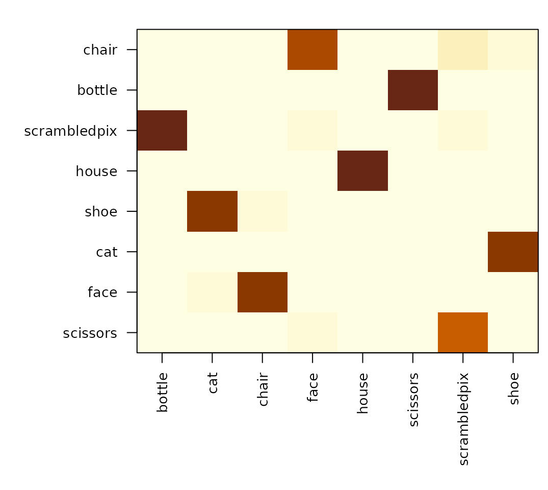

8-way confusion matrix in VT cortex (rows: observed category, columns: predicted). The diagonal shows that face and house come out cleanly while cat / shoe / bottle confuse with one another – the canonical Haxby 2001 pattern.

per_cat <- diag(prop.table(as.matrix(conf), margin = 1))
round(sort(per_cat, decreasing = TRUE), 2)
#> [1] 1.00 0.08 0.08 0.00 0.00 0.00 0.00 0.00

Faces and houses lead — exactly as in Figure 2 of the original paper.

Comparing classifiers

mvpa_model() reads its classifier from rMVPA’s pre-registered registry, so swapping the family is one line. Below we run the same VT analysis under five classifiers covering different inductive biases:

corclass — correlation-to-prototype, the original Haxby (2001) method.
naive_bayes — independent-feature Gaussian; a simple baseline.
rf — random forest (randomForest); ensemble of bagged trees.
svmLinear — linear support vector machine; large-margin separator.
sda_notune — shrinkage discriminant; rMVPA’s recommended default.

fit_one <- function(model_name, ...) {
  t0 <- Sys.time()
  mspec <- mvpa_model(load_model(model_name), dataset = ds, design = mvdes,
                      crossval = cval, ...)
  res <- run_regional(mspec, region_mask, verbose = FALSE)
  pt  <- res$performance_table
  data.frame(
    classifier = model_name,
    accuracy   = round(pt$Accuracy, 3),
    auc        = round(pt$AUC, 3),
    seconds    = round(as.numeric(difftime(Sys.time(), t0, units = "secs")), 1)
  )
}

panel <- rbind(
  fit_one("corclass"),
  fit_one("naive_bayes"),
  fit_one("rf",        tune_grid = data.frame(mtry = 50)),
  fit_one("svmLinear"),
  fit_one("sda_notune")
)
panel <- panel[order(-panel$accuracy), ]
panel
#>    classifier accuracy   auc seconds
#> 5  sda_notune    0.917 0.973     1.5
#> 4   svmLinear    0.698 0.853     2.1
#> 3          rf    0.500 0.694    10.4
#> 2 naive_bayes    0.375 0.481     1.7
#> 1    corclass    0.271 0.289     1.1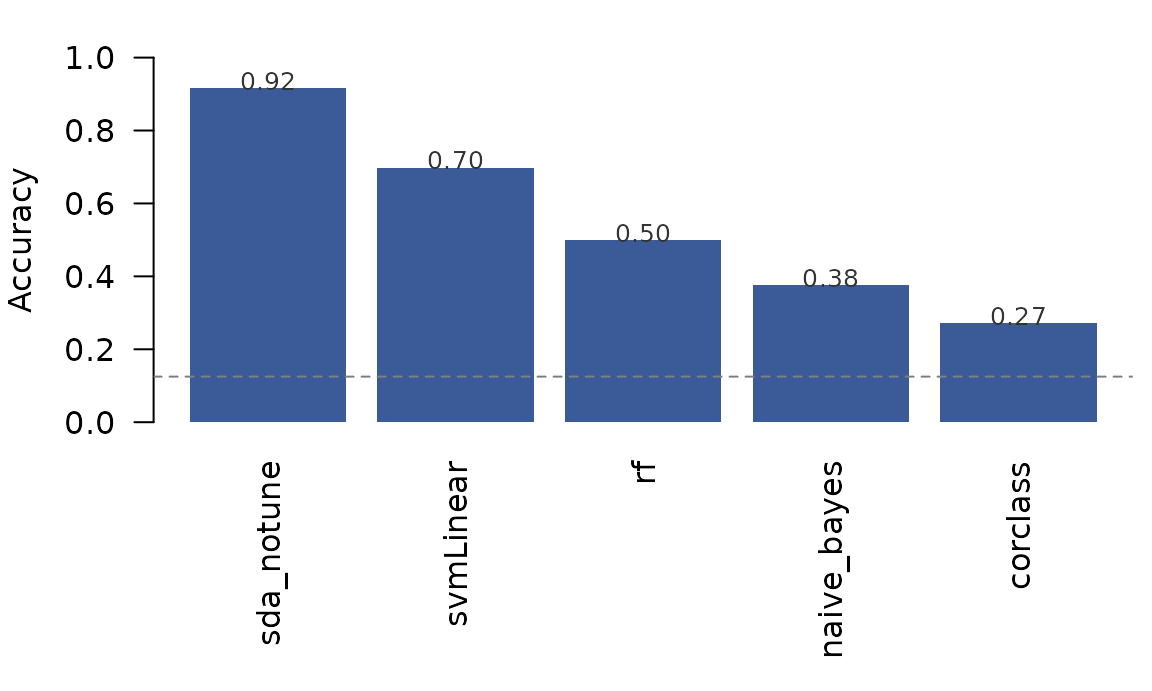

Cross-validated accuracy under five classifiers, all on the same VT patterns and the same leave-one-run-out CV. Dashed line = chance for an 8-way problem (12.5%).

sda_notune’s shrinkage discriminant dominates by ≈25 percentage points. That gap is not a cross-validation artefact: leave-one-run-out is honest here (each fold’s 8 test patterns come from a single held-out run; runs do not overlap; the bundled mean patterns are built per-run so no cross-run averaging leaks signal). Running sda::sda directly outside rMVPA on the same patterns and the same fold structure reproduces 0.917 to two decimal places.

Why such a wide spread? The dataset shape (96 observations × 577 voxels × 8 classes) is exactly the regime where pooled shrinkage covariance estimation pays for itself: voxels are strongly correlated, the within-class covariance is rank-deficient, and unregularised methods either overfit (naive_bayes is forced into independence; rf averages weak high-variance trees) or treat the boundary geometrically without using the covariance structure (svmLinear). corclass tops out at ≈27 % because it’s an 8-way correlation-to-prototype classifier; the canonical Haxby (2001) ≈90 % numbers came from a binary, split-half-within-run version of correlation classification that is structurally different from the 8-way leave-one-run-out reported here.

The full MVPAModels registry includes 22 classifiers; see ls(rMVPA:::MVPAModels) for the complete list and vignette("FeatureSelection") for adding feature selection inside the CV loop.

Where the raw data lives

The patterns.rds bundle in this package is one subject already collapsed to per-(category, run) mean patterns over the VT mask. If you want to start from raw BOLD and do your own preprocessing / first-level GLM, two routes:

A. The PyMVPA tutorial archive (≈300 MB) is the easiest source for the canonical preprocessed Subject 1 data with the published VT mask:

download.file(
  "http://data.pymvpa.org/datasets/haxby2001/subj1-2010.01.14.tar.gz",
  destfile = "subj1.tar.gz", mode = "wb"
)
untar("subj1.tar.gz")
# subj1/{bold.nii.gz, mask4_vt.nii.gz, labels.txt, anat.nii.gz, ...}

B. OpenNeuro ds000105 via the openneuro package for the raw BIDS layout (no preprocessing, no VT mask — bring your own pipeline):

library(openneuro)
res <- on_download(id = "ds000105", subjects = "sub-1")
# files are cached under on_cache_info()$path

The package’s data-raw/haxby2001_subj1.R script reproduces the bundled patterns.rds end-to-end from the PyMVPA archive.

Where to go next

For a searchlight version of this analysis, see vignette("Searchlight_Analysis"). The same mspec plus run_searchlight() produces a per-voxel decoding map.
For RSA-style geometry (rather than category labels), vignette("Kriegeskorte_92_Images") walks through the matched real-data RSA workflow.
For rMVPA’s classification ergonomics in general, see vignette("Regional_Analysis") and vignette("CrossValidation").

Citation

Haxby JV, Gobbini MI, Furey ML, Ishai A, Schouten JL, Pietrini P (2001). Distributed and overlapping representations of faces and objects in ventral temporal cortex. Science 293: 2425–2430. https://doi.org/10.1126/science.1063736

Subject 1 data are redistributed by the PyMVPA project and on OpenNeuro ds000105. Cite Haxby et al. (2001) and the data redistribution source you used.

Bradley Buchsbaum

2026-04-25

What this vignette is for

The bundled data

Wrap the patterns as an `mvpa_dataset`

Build the design and the model spec

Run the analysis

Cross-validated accuracy

The classic per-category pattern

Comparing classifiers

Where the raw data lives

Where to go next

Citation

Reproducing Haxby (2001) classification with rMVPA

Bradley Buchsbaum

2026-04-25

What this vignette is for

The bundled data

Wrap the patterns as an mvpa_dataset

Build the design and the model spec

Run the analysis

Cross-validated accuracy

The classic per-category pattern

Comparing classifiers

Where the raw data lives

Where to go next

Citation

Wrap the patterns as an `mvpa_dataset`