Advanced Regional MVPA Analysis in rMVPA

Introduction

Use regional MVPA when you already have an ROI mask and want one prediction summary per region. The input is a 4D neuroimaging dataset plus a design table; the output is a regional_mvpa_result containing cross-validated performance, trial-level predictions, and map-ready regional summaries.

This vignette follows one compact workflow: make a small dataset, define three ROIs, fit a blocked cross-validated classifier, and inspect the region-level performance.

Data Generation and Preparation

We begin by generating a synthetic volumetric dataset using the gen_sample_dataset() function. This function creates a 4D array (with spatial dimensions and multiple observations), along with a binary mask and an associated design for cross-validation.

data_out <- rMVPA::gen_sample_dataset(D = c(6,6,6), nobs = 80, blocks = 4, nlevels = 2)

data.frame(
  observations = length(data_out$design$block_var),
  active_voxels = sum(data_out$dataset$mask),
  blocks = length(unique(data_out$design$block_var)),
  classes = length(levels(data_out$design$targets))
)
#>   observations active_voxels blocks classes
#> 1           80           216      4       2

The returned list contains two objects:

dataset: an MVPA dataset object with training data and a binary mask.
design: an MVPA design object specifying the response variable and block structure.

Creating a Region Mask

For regional analysis, we need to define ROIs. Here, we create a region mask by randomly assigning each active voxel in the binary mask a region label (from 1 to 3). This simulates a scenario where the brain is partitioned into three regions of interest.

mask <- data_out$dataset$mask
nvox <- sum(mask)

set.seed(123)
region_mask <- neuroim2::NeuroVol(
  sample(1:3, size = nvox, replace = TRUE),
  neuroim2::space(mask),
  indices = which(mask > 0)
)
table(region_mask)
#> region_mask
#>  1  2  3 
#> 69 74 73

Setting Up the MVPA Model

Next, we create an MVPA model to evaluate a classification task. In brief, we construct an mvpa_dataset, specify the design (including the block variable and response), and define the model with mvpa_model() using a chosen classifier and cross‑validation strategy.

dset <- mvpa_dataset(data_out$dataset$train_data, mask = data_out$dataset$mask)
cval <- blocked_cross_validation(data_out$design$block_var)

mod <- load_model("sda")
tune_grid <- data.frame(lambda = 0.01, diagonal = FALSE)

mvpa_mod <- mvpa_model(
  mod,
  dataset = dset,
  design = data_out$design,
  crossval = cval,
  tune_grid = tune_grid
)
mvpa_mod
#> mvpa_model object. 
#> model:  sda 
#> model type:  classification 
#> tune_reps:  15 
#> tune_grid:  
#>   lambda diagonal
#> 1   0.01    FALSE
#> 
#>  Blocked Cross-Validation 
#> 
#> - Dataset Information 
#>   - Observations:  80 
#>   - Number of Folds:  4 
#> - Block Information 
#>   - Total Blocks:  4 
#>   - Mean Block Size:  20  (SD:  0 ) 
#>   - Block Sizes:  1: 20, 2: 20, 3: 20, 4: 20 
#> 
#> 
#>  MVPA Dataset 
#> 
#> - Training Data 
#>   - Dimensions:  6 x 6 x 6 x 80 observations 
#>   - Type:  DenseNeuroVec 
#> - Test Data 
#>   -  None 
#> - Mask Information 
#>   - Areas:  TRUE : 216 
#>   - Active voxels/vertices:  216 
#> 
#> 
#>  MVPA Design 
#> 
#> - Training Data 
#>   - Observations:  80 
#>   - Response Type:  Factor
#>   - Levels:  a, b 
#>   - Class Distribution:  a: 40, b: 40 
#> - Test Data 
#>   -  None 
#> - Structure 
#>   - Blocking:  Present
#>   - Number of Blocks:  4 
#>   - Mean Block Size:  20  (SD:  0 ) 
#>   - Split Groups:  None

The model object packages the dataset, design, classifier, tuning grid, and cross-validation plan.

Running the Regional Analysis

The regional analysis is executed with run_regional(). Internally it prepares ROI indices from the region mask, applies the MVPA model to each ROI, and then compiles performance metrics and prediction tables.

regional_results <- run_regional(mvpa_mod, region_mask)

The output is a regional_mvpa_result object with a performance_table (cross‑validated metrics per region), a prediction_table (trial‑level predictions), and vol_results (volumetric maps of performance across the brain).

Examining the Results

We can inspect the performance table to evaluate model accuracy in each region.

regional_results$performance_table
#> # A tibble: 3 × 3
#>   roinum Accuracy      AUC
#>    <int>    <dbl>    <dbl>
#> 1      1    0.575  0.188  
#> 2      2    0.488  0.00125
#> 3      3    0.488 -0.157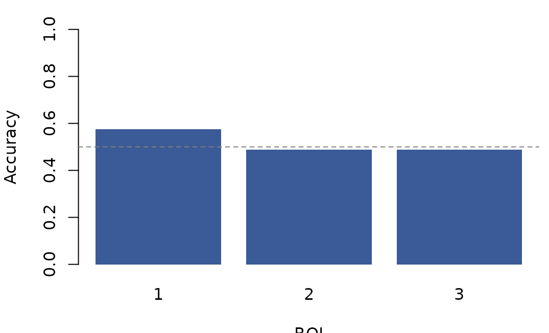

Cross-validated accuracy per region. The dashed line marks chance for a 2-class problem.

The bar plot makes between-region differences visible at a glance and shows where each region sits relative to chance. For a compact trial-level check, show the first few predictions:

utils::head(regional_results$prediction_table)
#> # A tibble: 6 × 8
#> # Rowwise: 
#>   .rownum roinum observed pobserved predicted correct prob_a  prob_b
#>     <int>  <int> <fct>        <dbl> <fct>     <lgl>    <dbl>   <dbl>
#> 1       1      1 b           0.872  b         TRUE    0.128  0.872  
#> 2       2      1 a           0.961  a         TRUE    0.961  0.0393 
#> 3       3      1 a           0.996  a         TRUE    0.996  0.00371
#> 4       4      1 b           0.983  b         TRUE    0.0166 0.983  
#> 5       5      1 b           0.0243 a         FALSE   0.976  0.0243 
#> 6       6      1 a           0.805  a         TRUE    0.805  0.195

Volumetric results (vol_results) can be further visualized with neuroimaging tools to determine spatial patterns of performance.

Summary

This vignette showed you how to generate synthetic neuroimaging data, define ROIs with region masks, set up MVPA models with cross-validation, run analyses across ROIs, and interpret the performance metrics. You now have the tools to conduct regional MVPA analyses on your own neuroimaging data.

For further details, see vignette("Searchlight_Analysis") for the searchlight counterpart and vignette("CrossValidation") for cross-validation strategies.

Bradley Buchsbaum