Design-Subspace Summaries for Task PLS
Source:vignettes/task-design-subspace.Rmd
task-design-subspace.RmdTask PLS gives you latent variables over a flattened set of group-by-condition cells. When the conditions come from a factorial design, the next question is often more specific: does the covariance pattern live mostly in a task effect, a group-by-task interaction, or a higher-order term?
The design-subspace helpers answer that question on the design side of Task PLS. They do not run voxelwise ANOVAs. They build factorial subspaces over the same centered cell rows used by Task PLS and summarize how much cross-block covariance lies in each subspace.
What are the data?
This example uses synthetic data with two groups, two tasks, and two levels. The planted signal includes a group-by-task effect, a level effect, and a smaller three-way interaction.
The condition key maps each PLS condition label back to the factors that created it.
condition_key
#>    condition  task level
#> 1  recog_low recog   low
#> 2 recog_high recog  high
#> 3  nback_low nback   low
#> 4 nback_high nback  high
How do we keep the Task PLS cross-block matrix?
Design-subspace summaries need the cell-level cross-block matrix used
by Task PLS before the singular value decomposition. Request it at fit
time with keep_crossblock = TRUE.
spec <- pls_spec() |>
  add_subjects(list(control, sdam), groups = c(n_subjects, n_subjects)) |>
  add_conditions(nrow(condition_key), labels = condition_key$condition) |>
  add_group_labels(c("control", "sdam")) |>
  configure(method = "task", meancentering = "grand_mean")

fit <- run(spec, progress = FALSE, keep_crossblock = TRUE)
The ordinary Task PLS result is still a latent-variable model. The new field is only a compact summary object needed for design-subspace calculations; it does not store the original subject-level imaging data.
How do we define the factorial design?
Use pls_design() to describe the design over
group-condition cells. The rows come from the PLS result; the
condition-level factors come from the condition key.
design <- pls_design(
  ~ group * task * level,
  condition_key = condition_key,
  between = "group",
  within = c("task", "level")
)
You can inspect the cell table to confirm the row order. These are the rows of the Task PLS cross-block matrix: all conditions for group 1, then all conditions for group 2.
design_cell_table(fit, design = design)[
  , c("row_index", "group", "condition", "task", "level")
]
#>     row_index   group  condition  task level
#> 1           1 control  recog_low recog   low
#> 2           2 control recog_high recog  high
#> 3           3 control  nback_low nback   low
#> 4           4 control nback_high nback  high
#> 1.1         5    sdam  recog_low recog   low
#> 2.1         6    sdam recog_high recog  high
#> 3.1         7    sdam  nback_low nback   low
#> 4.1         8    sdam nback_high nback  high
Which factorial terms does an LV resemble?
Start descriptively. decompose_design_terms() projects
one design-side LV onto the centered factorial subspaces and reports how
much LV energy aligns with each term. This helps interpret an already
selected LV; it is not a p-value.
lv_terms <- decompose_design_terms(fit, lv = 1, design = design)
lv_terms$fraction <- round(lv_terms$fraction, 3)
lv_terms[order(lv_terms$fraction, decreasing = TRUE),
         c("term", "rank", "fraction")]
#>               term rank fraction
#> 5      group:level    1    0.855
#> 1            group    1    0.110
#> 2             task    1    0.022
#> 6       task:level    1    0.010
#> 3            level    1    0.001
#> 4       group:task    1    0.000
#> 7 group:task:level    1    0.000
For this simulated example, LV1 should align strongly with the planted factorial effects. The exact ordering is data-dependent because the example still includes noise.
A plot of the same LV-level decomposition is useful when you want a quick interpretive summary for a selected latent variable.
plot_design_contrasts(fit, lv = 1, condition_key = condition_key)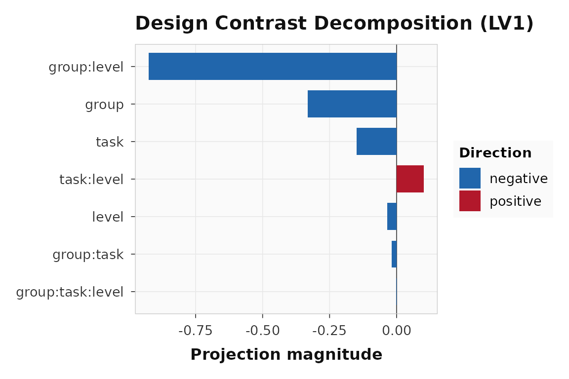
Effect-coded decomposition of the LV1 design scores.
How do we fit term-specific PLS components?
The ASCA-like step is design_subspace_svd(). It projects
the stored Task PLS cross-block matrix into each centered factorial
subspace, then fits a separate SVD for each term. This is a fitted
term-specific PLS decomposition, not a post-hoc label attached to a
global LV.
term_fit <- design_subspace_svd(
  fit,
  design = design,
  ncomp = 2,
  statistic = "trace"
)

term_fit$statistics[, c("term", "rank", "trace", "largest_root")]
#>               term rank    trace largest_root
#> 1            group    1 2.884746     2.884746
#> 2             task    1 2.780662     2.780662
#> 3            level    1 2.727144     2.727144
#> 4       group:task    1 2.227952     2.227952
#> 5      group:level    1 4.749049     4.749049
#> 6       task:level    1 2.735260     2.735260
#> 7 group:task:level    1 3.228667     3.228667
components <- term_fit$components
components$percent_term_covariance <- round(components$percent_term_covariance, 3)
components[components$component == 1,
           c("term", "component", "singular_value", "percent_term_covariance")]
#>               term component singular_value percent_term_covariance
#> 1            group         1       1.698454                       1
#> 2             task         1       1.667532                       1
#> 3            level         1       1.651407                       1
#> 4       group:task         1       1.492632                       1
#> 5      group:level         1       2.179231                       1
#> 6       task:level         1       1.653862                       1
#> 7 group:task:level         1       1.796849                       1
The term-level trace is the total squared singular-value
energy in that subspace. largest_root is the dominant
PLS-like component for the same projected matrix.
Can we get resampling p-values?
Yes, against an explicitly named null.
test_design_subspaces() recomputes each subspace statistic
over permuted Task PLS cross-block matrices and returns a p-value per
term.
The only null currently implemented is
permutation = "global_task_pls" — the same permutation
scheme that ordinary Task PLS already uses for LV significance.
Concretely, for each permutation the routine
- permutes condition labels within each subject and permutes subjects
across groups (
pls_perm_order()), - rebuilds the centered group-by-condition cross-block matrix from the
permuted subject rows (
pls_get_covcor()), and - recomputes each term-subspace statistic on the permuted cross-block.
Under this null every factorial label is broken simultaneously — there is no group structure, no task structure, no interaction structure. The question being asked for each term is therefore:
Is the covariance projected into this term’s subspace larger than what we would see if subject-condition labels were exchangeable?
That is the right null for an omnibus “is this term doing
anything?” question, and it is the standard PLS permutation null
restricted to a subspace. It is not a nested test: it
cannot tell you whether group:task adds anything
beyond group, because the same permutation that
breaks group:task also breaks group. A
reduced-model-preserving null (Freedman–Lane–style) is the right tool
for nested questions and is filed as future work.
The correction = "maxT" option compares each observed
term statistic to the per-permutation maximum across all terms, giving
family-wise adjusted p-values across the table.
set.seed(20260510)
term_tests <- test_design_subspaces(
  spec,
  fit = fit,
  design = design,
  statistic = "trace",
  nperm = 99,
  permutation = "global_task_pls",
  correction = "maxT"
)
term_tests$share <- round(term_tests$statistic / sum(term_tests$statistic), 3)
term_tests$statistic <- round(term_tests$statistic, 2)
term_tests[, c("term", "rank", "statistic", "share", "p_value", "p_adjusted")]
#>               term rank statistic share   p_value p_adjusted
#> 1            group    1      2.88 0.135 0.5454545  1.0000000
#> 2             task    1      2.78 0.130 0.7979798  1.0000000
#> 3            level    1      2.73 0.128 0.8080808  1.0000000
#> 4       group:task    1      2.23 0.104 0.9797980  1.0000000
#> 5      group:level    1      4.75 0.223 0.1616162  0.7272727
#> 6       task:level    1      2.74 0.128 0.8080808  1.0000000
#> 7 group:task:level    1      3.23 0.151 0.5858586  0.9898990
If you want the most PLS-like single-root statistic instead of
omnibus energy, use statistic = "largest_root".
largest_root <- test_design_subspaces(
  fit,
  design = design,
  statistic = "largest_root"
)
largest_root$statistic <- round(largest_root$statistic, 2)
largest_root[, c("term", "rank", "statistic")]
#>               term rank statistic
#> 1            group    1      2.88
#> 2             task    1      2.78
#> 3            level    1      2.73
#> 4       group:task    1      2.23
#> 5      group:level    1      4.75
#> 6       task:level    1      2.74
#> 7 group:task:level    1      3.23
How do we ask a nested design question?
Use compare_design_subspaces() when your question is
“what is added by the full model beyond the reduced model?” The function
residualizes the full design against the reduced design in the same
centered Task PLS row space, then fits the delta-subspace SVD.
task_beyond_group <- compare_design_subspaces(
  spec,
  fit = fit,
  design = design,
  reduced = ~ group,
  full = ~ group * task,
  nperm = 99,
  permutation = "global_task_pls"
)

interactions_beyond_main_effects <- compare_design_subspaces(
  spec,
  fit = fit,
  design = design,
  reduced = ~ group + task + level,
  full = ~ group * task * level,
  nperm = 99,
  permutation = "global_task_pls"
)

nested_tests <- rbind(task_beyond_group, interactions_beyond_main_effects)
nested_tests$statistic <- round(nested_tests$statistic, 2)
nested_tests[, c("reduced", "full", "added_terms", "rank", "statistic", "p_value")]
#>                 reduced                  full
#> 1                ~group         ~group * task
#> 2 ~group + task + level ~group * task * level
#>                                                added_terms rank statistic
#> 1                                        task + group:task    3      7.89
#> 2 group:task + group:level + task:level + group:task:level    7     21.26
#>     p_value
#> 1 0.9696970
#> 2 0.9494949
The statistic column is the observed covariance
energy in the residualized delta subspace — i.e., the part of the full
design that is orthogonal to the reduced design after centering. This
part of the answer is purely descriptive and does not depend on the
permutation null.
The p_value column, however, again uses the
"global_task_pls" null. That is, the delta statistic is
compared to the distribution of delta statistics computed on cross-block
matrices where all subject-condition labels have been permuted
— not just the labels associated with the added terms. So the p-value
answers:
Is the energy in the full-minus-reduced subspace larger than expected when there is no design structure at all?
That is informative and it is what classical Task PLS already gives
you for an LV. It is not the same as testing “does
adding task and group:task improve fit beyond
group alone” in the strict nested sense: a true nested test
would permute under a null that preserves the reduced model, and that
null is not yet implemented. Use the descriptive statistic
and rank columns when you want to compare the size
of the added subspace, and treat the p-value as global-null evidence
that something in the delta subspace is non-trivial.
How should the summaries be interpreted?
Keep four distinctions clear:
-
plot_scores()andplot_design_contrasts()help you interpret selected LVs. -
decompose_design_terms()descriptively attributes one LV’s design vector to factorial terms. -
design_subspace_svd()fits term-specific PLS components from projected cross-block matrices. -
test_design_subspaces()andcompare_design_subspaces()add observed statistics and, when apls_specis available, global Task PLS permutation p-values.
These are design-subspace summaries, not classical ANOVA tables and not voxelwise tests. They differ from classical ANOVA in three ways worth keeping in mind:
- The response is multivariate. The statistic is squared singular-value energy of a projected cross-block matrix, not a univariate sum-of-squares. There is no F ratio and no residual mean square; the reference distribution is built by permutation, not by Gaussian-error theory.
- The null is exchangeability of subject-condition labels. It is the same null used for LV significance in ordinary Task PLS — labels are permuted, cross-blocks are rebuilt, statistics are recomputed. There is no independence or homoscedasticity assumption.
-
Term tests are global, not sequential. The
currently implemented null breaks all design structure at once. Each
term’s p-value answers “is this subspace doing anything?” against a
no-design null, not “does this term add anything beyond the others?” The
latter is what nested
compare_design_subspaces()calls would ask once a reduced-model-preserving null is implemented.
Treated this way, the table is a multivariate, design-aware companion to the LV table — not a substitute for ANOVA and not a voxelwise test.
Where to go next
Use vignette("sdam-firstlevel-task-pls") for a
first-level image-map example with design-score heatmaps and contrast
plots. Use ?pls_design,
?decompose_design_terms, ?design_subspace_svd,
?test_design_subspaces, and
?compare_design_subspaces for the function-level
reference.