Predictive Measures and Resampling Inference • plsrri

library(plsrri)

You can now ask two different questions of the same PLS analysis. First, does the latent-variable decomposition look non-random and stable under the usual PLS resampling tools? Second, can the fitted score space support honest out-of-fold prediction for held-out subjects? plsrri now supports both.

This article shows how predictive measures complement, rather than replace, the existing permutation, bootstrap, and split-half analyses:

permutation on a pls_result asks whether an LV is stronger than expected under the null decomposition
bootstrap asks which voxel or behavior relationships are stable
predictive cross-validation asks whether the learned score space generalizes to held-out subjects

What does a predictive quick win look like?

This vignette uses one synthetic brain-behavior dataset throughout. The quick win is a classification analysis: can you recover a held-out high-vs-low subject label from the score space learned inside each training fold?

round_numeric_df(cls_result$summary)
#>     metric mean   sd
#> 1 accuracy 0.79 0.08
#> 2      auc 0.82 0.07

round_numeric_df(cls_result$boot_ci[, c("metric", "estimate", "lower", "upper")])
#>            metric estimate lower upper
#> accuracy accuracy     0.79  0.53  0.94
#> auc           auc     0.81  0.60  0.97

The key point is that this object is not another decomposition summary. It is an out-of-fold predictive result built from nested cross-validation, with its own permutation null and bootstrap intervals.

What data are we using?

The example has 24 subjects, 2 conditions, 90 features, and two behavior measures. One subject-level latent factor drives a brain block, the symptom measure, and the binary diagnosis; a second block captures condition structure.

rbind(
  brain = dim(brain),
  behavior = dim(behav)
)
#>          [,1] [,2]
#> brain      48   90
#> behavior   48    2

head(data.frame(
  subject = seq_len(6),
  symptom_score = round(symptom_score[1:6], 2),
  diagnosis = diagnosis[1:6]
))
#>   subject symptom_score diagnosis
#> 1       1         -1.37       low
#> 2       2         -1.49       low
#> 3       3         -1.15       low
#> 4       4         -1.03       low
#> 5       5         -1.04       low
#> 6       6         -1.33       low

What does ordinary PLS inference tell you first?

Start with the decomposition-side questions. Here the behavior PLS fit asks whether there is a dominant brain-behavior latent variable, and whether the behavior links are stable under bootstrap resampling.

round(cbind(
  pvalue = significance(fit),
  variance = singular_values(fit, normalize = TRUE)
), 2)
#>     pvalue variance
#> LV1      0    74.80
#> LV2      0    24.97
#> LV3      1     0.15
#> LV4      1     0.09

plot_singular_values(fit)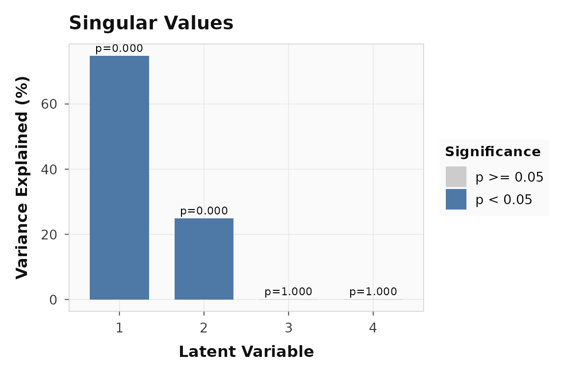

The decomposition-side permutation test is about latent variables, not held-out prediction. LV1 dominates the singular value spectrum.

LV1 is clearly non-null in the ordinary PLS sense. That still does not tell you whether held-out subjects can be predicted. It only tells you that the brain-behavior decomposition is stronger than the null decomposition generated by row shuffling.

Bootstrap intervals answer a different question again: which specific brain-behavior links are stable?

round_numeric_df(corr_table)
#>               loading lower upper
#> 1  baseline / symptom -0.96 -0.79
#> 2  baseline / reserve  0.89  0.97
#> 3 challenge / symptom -0.97 -0.86
#> 4 challenge / reserve  0.93  0.98

All four behavior-by-condition intervals stay away from zero. That supports the claim that the symptom/reserve pattern is stable, but it is still not a held-out predictive statement.

What does predictive regression add?

Now switch from decomposition inference to honest prediction. The regression target is the subject-level symptom score, not the repeated behavior matrix used to fit the decomposition.

round_numeric_df(reg_result$summary)
#>   metric mean   sd
#> 1   rmse 0.53 0.10
#> 2    mae 0.45 0.08
#> 3    rsq 0.67 0.15

round_numeric_df(reg_result$boot_ci[, c("metric", "estimate", "lower", "upper")])
#>      metric estimate lower upper
#> rmse   rmse     0.53  0.39  0.67
#> mae     mae     0.45  0.34  0.58
#> rsq     rsq     0.70  0.48  0.83

For speed, this vignette uses only 9 predictive label permutations, so the smallest attainable predictive p-value is 0.1. In a real analysis you would increase this substantially.

reg_result$perm_test
#> $metric
#> [1] "rmse"
#> 
#> $observed
#> [1] 0.5251243
#> 
#> $null_distribution
#> [1] 1.0656167 1.1893644 1.3808130 0.9353916 1.1422777 1.1948747 1.1586831
#> [8] 1.2519858 1.1399975
#> 
#> $p_value
#> [1] 0.1
#> 
#> $num_perm
#> [1] 9

The continuous outcome is recoverable out of sample: the held-out R^2 is 0.67, and the observed RMSE is smaller than the median value from the shuffled-label null.

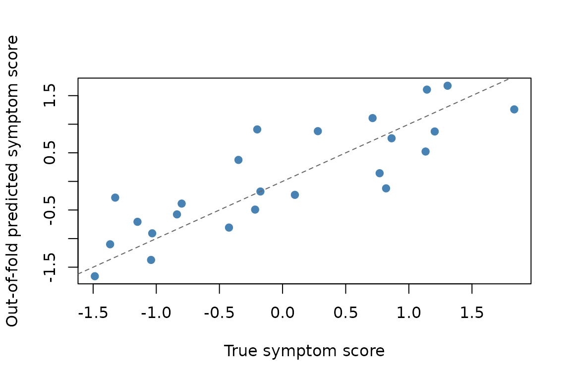
Each point is one held-out subject, aggregated across outer folds. Predictive validation asks whether these subject-level estimates track the true outcome.

What does predictive classification add?

The same score space can also be used for classification. Here the target is a binary high-vs-low diagnosis derived from the same latent factor.

round_numeric_df(cls_result$summary)
#>     metric mean   sd
#> 1 accuracy 0.79 0.08
#> 2      auc 0.82 0.07

cls_result$perm_test
#> $metric
#> [1] "accuracy"
#> 
#> $observed
#> [1] 0.7916667
#> 
#> $null_distribution
#> [1] 0.4583333 0.5833333 0.5000000 0.6666667 0.6666667 0.5000000 0.5416667
#> [8] 0.5000000 0.4583333
#> 
#> $p_value
#> [1] 0.1
#> 
#> $num_perm
#> [1] 9

round_numeric_df(cls_result$boot_ci[, c("metric", "estimate", "lower", "upper")])
#>            metric estimate lower upper
#> accuracy accuracy     0.79  0.53  0.94
#> auc           auc     0.81  0.60  0.97

Again, the predictive inference is about held-out performance. Accuracy and AUC are computed from out-of-fold predictions, and the predictive permutation test compares those numbers to a null generated by re-running the full nested cross-validation workflow with shuffled subject labels.

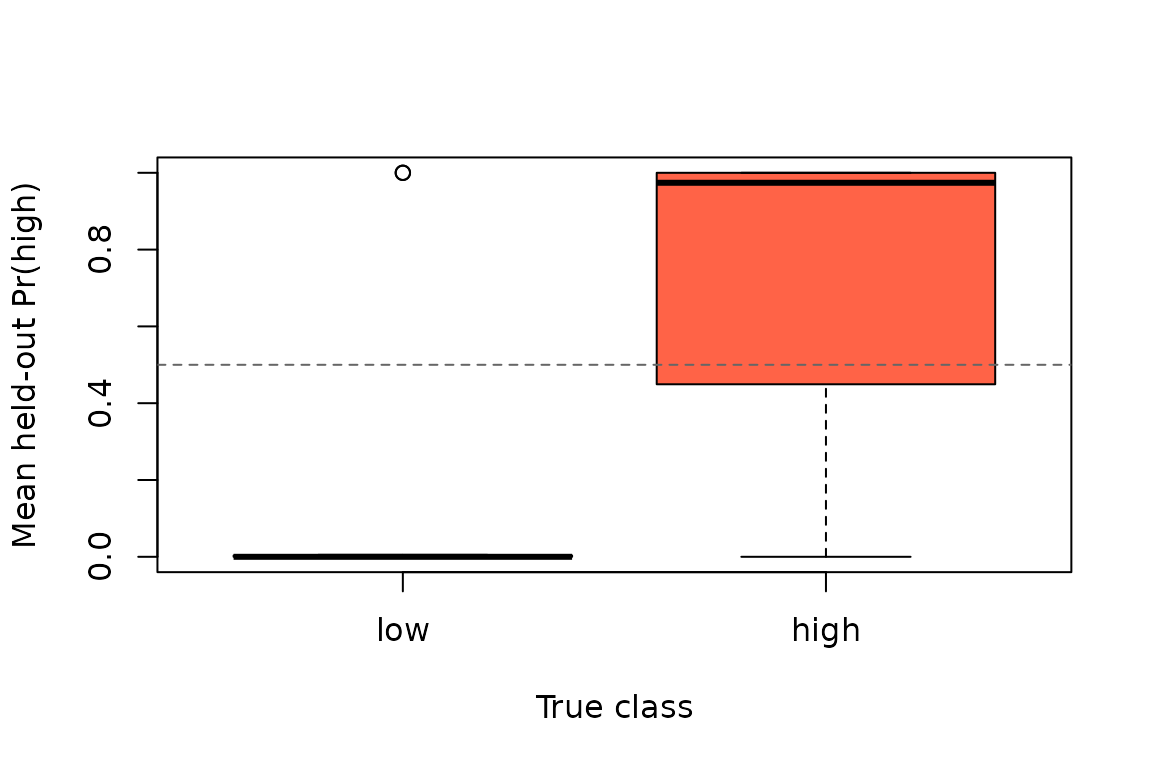
Held-out class probabilities aggregated to one row per subject. The horizontal line marks a 0.5 decision threshold.

How do the inferential layers complement each other?

These tools are strongest when you treat them as complementary rather than interchangeable:

comparison
#>                                                              question
#> 1 Is the dominant latent variable stronger than a null decomposition?
#> 2 Which behavior relationships are stable under bootstrap resampling?
#> 3   Can the latent score space predict a held-out continuous outcome?
#> 4              Can the latent score space classify held-out subjects?
#>                                              diagnostic
#> 1 LV1 permutation p = 0.000; variance explained = 74.8%
#> 2                4 of 4 behavior intervals exclude zero
#> 3                           OOF R^2 = 0.67; RMSE = 0.53
#> 4                       OOF accuracy = 0.79; AUC = 0.82

You can read the table as four distinct questions:

Decomposition permutation: is there a latent variable stronger than a null PLS decomposition?
Decomposition bootstrap: which loadings or correlations are stable?
Predictive regression/classification: do those learned score patterns generalize to held-out subjects?

Split-half validation fits beside the first two, not the last one. It asks whether the decomposition itself replicates across random halves of the data, while evaluate_prediction() asks whether a training-fit score space supports honest out-of-fold prediction.

Where should you go next?

Goal	Resource
Core task PLS workflow	`vignette("plsrri")`
Ordinary behavior PLS workflow	`vignette("behavior-pls")`
Multiblock and seed methods	`vignette("multiblock-and-seed")`
Predictive entry point	`?evaluate_prediction`
Decomposition-side significance	`?significance`
Bootstrap confidence intervals	`?confidence`