Displaying Surfaces with RGL

This vignette demonstrates how to display 3D brain surface meshes using the rgl plotting tools provided by the neurosurf package, primarily through the plot() method which utilizes the view_surface() function internally.

For interactive HTML widgets, see Interactive Surface Visualization with surfwidget. For high-level, surfplot-style multi-view layouts with shared colourbars and atlas outlines, see Surfplot-style Figures with neurosurf.

Setup and Loading Data

First, we set up knitr options to embed rgl plots directly into the HTML output using WebGL and prevent standalone rgl windows from popping up during knitting. We then load example left and right hemisphere white matter surfaces included with the package and prepare some data (smoothed geometry, curvature, random values) for the examples.

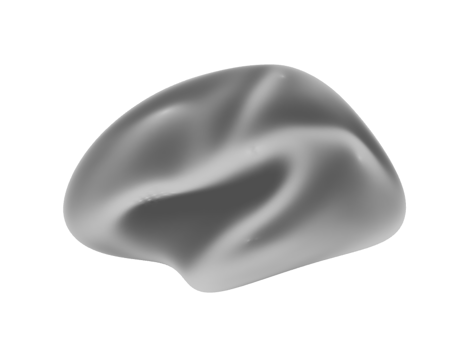
Basic Surface Plotting

The simplest way to display a SurfaceGeometry object is using the plot() method. By default, it renders the surface with a light gray background. We can specify a viewpoint.

# Plot the smoothed left hemisphere from a lateral viewpoint
render_surface(white_lh_display, viewpoint = "lateral", lit = TRUE)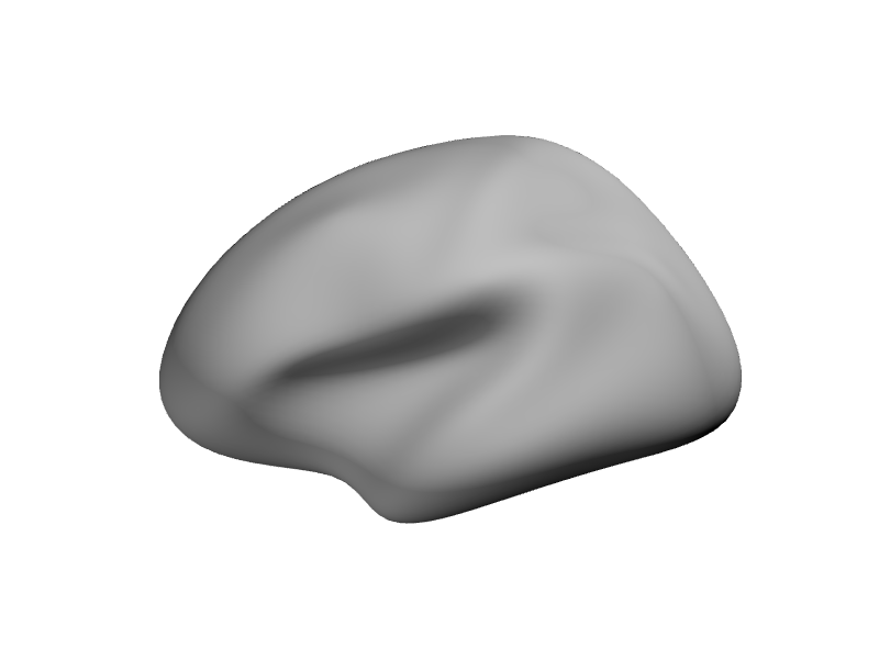
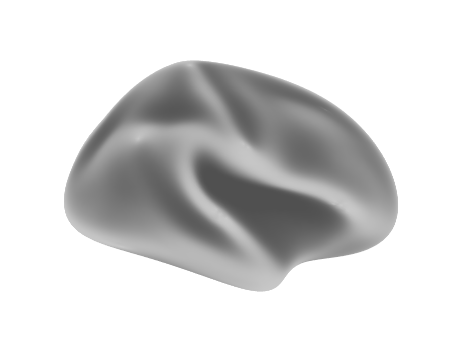
#> Warning in min(x): no non-missing arguments to min; returning Inf
#> Warning in max(x): no non-missing arguments to max; returning -Inf
#> file:////private/var/folders/9h/nkjq6vss7mqdl4ck7q1hd8ph0000gp/T/Rtmp8JJqZZ/file1688a3c77c33.html screenshot completed

Coloring Based on Curvature

Surface curvature helps distinguish gyri (outward folds) from sulci (inward folds). The curvature() function calculates this, and curv_cols() provides a simple binary color mapping (default: light gray for positive/gyri, dark gray for negative/sulci). We can pass these colors to the bgcol argument of plot() to color the surface background.

# Calculate curvature colors
curv_colors <- curv_cols(curv_lh_display)

# Plot with curvature background from a medial viewpoint
render_surface(white_lh_display, bgcol = curv_colors, viewpoint = "medial", specular = "black")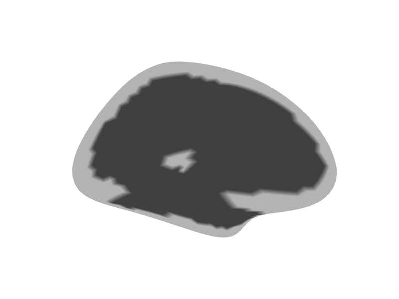
#> Warning in min(x): no non-missing arguments to min; returning Inf
#> Warning in max(x): no non-missing arguments to max; returning -Inf
#> file:////private/var/folders/9h/nkjq6vss7mqdl4ck7q1hd8ph0000gp/T/Rtmp8JJqZZ/file1688a17ad03c.html screenshot completed

Overlaying Data Values

Often, we want to visualize data mapped onto the surface vertices (e.g., activation values, thickness). We can pass a vector of values to the vals argument. The cmap argument specifies the color map, and irange defines the data range to map onto the colormap. Values outside irange are clamped to the minimum or maximum color.

# Overlay random data using a rainbow colormap
# Map data range from -2 to 2 onto the colormap
render_surface(white_lh_display, vals = random_vals_display_smooth, cmap = rainbow(256),
               irange = c(-2, 2), thresh = NULL, viewpoint = "lateral", specular = "gray")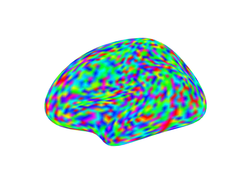
#> file:////private/var/folders/9h/nkjq6vss7mqdl4ck7q1hd8ph0000gp/T/Rtmp8JJqZZ/file1688a21050e9e.html screenshot completed

Thresholding Data Visualization

The thresh argument (a vector of two values, c(lower, upper)) can be used with vals to make parts of the surface transparent. Vertices where the corresponding value in vals is inside this range (between lower and upper) are rendered transparently; values outside remain opaque. This is useful for masking out a band of values.

# Same data overlay as above, but make values between -1 and 1 transparent
render_surface(white_lh_display, vals = random_vals_display_smooth, cmap = rainbow(256),
               irange = c(-2, 2), thresh = c(-1, 1), viewpoint = "lateral", lit = TRUE)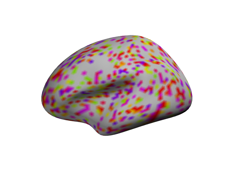
#> file:////private/var/folders/9h/nkjq6vss7mqdl4ck7q1hd8ph0000gp/T/Rtmp8JJqZZ/file1688a2f00b8b6.html screenshot completed

Direct Vertex Coloring

Instead of mapping data values to a colormap, you can provide a vector of specific hex color codes directly to the vert_clrs argument. This overrides vals and cmap. The vector length must match the number of vertices.

# Color vertices based on their x-coordinate (e.g., red for positive x, blue for negative)
x_coords <- coords(white_lh_display)[, 1]
vertex_colors <- ifelse(x_coords > median(x_coords), "#FF0000", "#0000FF") # Red/Blue

render_surface(white_lh_display, vert_clrs = vertex_colors, viewpoint = "ventral", lit = TRUE)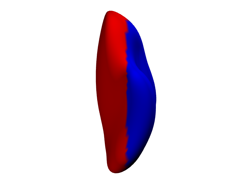
#> Warning in min(x): no non-missing arguments to min; returning Inf
#> Warning in max(x): no non-missing arguments to max; returning -Inf
#> file:////private/var/folders/9h/nkjq6vss7mqdl4ck7q1hd8ph0000gp/T/Rtmp8JJqZZ/file1688a4154d74f.html screenshot completed

Controlling Transparency

The alpha argument controls the overall transparency of the surface, ranging from 0 (fully transparent) to 1 (fully opaque).

# Plot the surface with 60% opacity (40% transparent)
render_surface(white_lh_display, vals = random_vals_display_smooth, cmap = heat.colors(256),
               irange = c(-2, 2), alpha = 0.6, viewpoint = "posterior")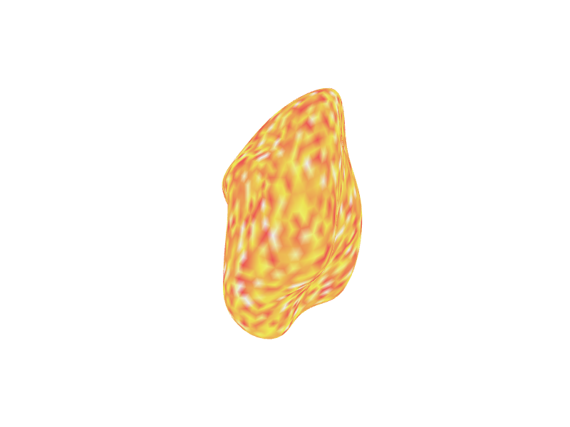
#> file:////private/var/folders/9h/nkjq6vss7mqdl4ck7q1hd8ph0000gp/T/Rtmp8JJqZZ/file1688a1c69f6f7.html screenshot completed

Adjusting Lighting and Material

The appearance of the surface is affected by lighting. The specular argument controls the color of specular highlights (shininess). Setting it to "black" creates a matte appearance.

# Plot with a matte finish (no specular highlights)
render_surface(white_lh_display, vals = random_vals_display_smooth, cmap = topo.colors(256),
               irange = c(-2, 2), specular = "black", viewpoint = "lateral", lit = TRUE)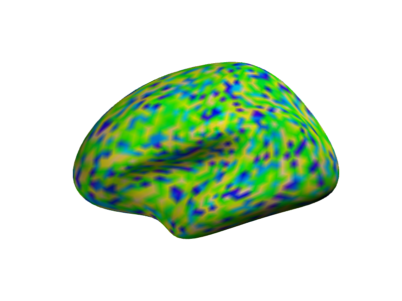
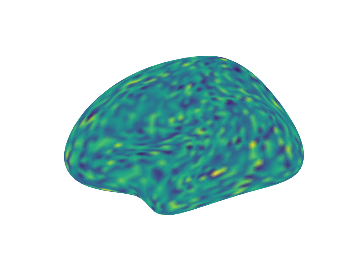
#> file:////private/var/folders/9h/nkjq6vss7mqdl4ck7q1hd8ph0000gp/T/Rtmp8JJqZZ/file1688a7c98a76.html screenshot completed

Snapshotting to an image (for knitr/CI)

Use to render an off-screen PNG and include it directly:

.render_counter$n <- .render_counter$n + 1
snapshot_file <- knitr::fig_path(paste0("-snapshot-", .render_counter$n, ".png"))
dir.create(dirname(snapshot_file), recursive = TRUE, showWarnings = FALSE)

img_path <- try(snapshot_surface(white_lh_display,
                                 file = snapshot_file,
                                 vals = random_vals_display_smooth,
                                 cmap = viridis::viridis(256),
                                 viewpoint = "lateral",
                                 specular = "black",
                                 width = 1200, height = 900),
                silent = TRUE)
#> file:////private/var/folders/9h/nkjq6vss7mqdl4ck7q1hd8ph0000gp/T/Rtmp8JJqZZ/file1688a4319fa86.html screenshot completed

if (!inherits(img_path, "try-error") && is.character(img_path) && file.exists(img_path)) {
  knitr::include_graphics(img_path)
} else {
  cat("*(Snapshot unavailable in this build environment)*")
}

Changing Viewpoints

The viewpoint argument can be set to common anatomical views like "lateral", "medial", "ventral", or "posterior". The function automatically selects the correct left/right version based on the surface’s hemisphere information (surf@hemi).

# Display multiple viewpoints
render_multi_view(white_lh_display, viewpoints = c("lateral", "medial", "ventral", "posterior"))
#> Warning in min(x): no non-missing arguments to min; returning Inf
#> Warning in max(x): no non-missing arguments to max; returning -Inf
#> file:////private/var/folders/9h/nkjq6vss7mqdl4ck7q1hd8ph0000gp/T/Rtmp8JJqZZ/file1688a5dd5293b.html screenshot completed
#> Warning in min(x): no non-missing arguments to min; returning Inf
#> Warning in min(x): no non-missing arguments to max; returning -Inf
#> file:////private/var/folders/9h/nkjq6vss7mqdl4ck7q1hd8ph0000gp/T/Rtmp8JJqZZ/file1688a5586109d.html screenshot completed
#> Warning in min(x): no non-missing arguments to min; returning Inf
#> Warning in min(x): no non-missing arguments to max; returning -Inf
#> file:////private/var/folders/9h/nkjq6vss7mqdl4ck7q1hd8ph0000gp/T/Rtmp8JJqZZ/file1688a54acdf48.html screenshot completed
#> Warning in min(x): no non-missing arguments to min; returning Inf
#> Warning in min(x): no non-missing arguments to max; returning -Inf
#> file:////private/var/folders/9h/nkjq6vss7mqdl4ck7q1hd8ph0000gp/T/Rtmp8JJqZZ/file1688a21771b66.html screenshot completed

Displaying Two Hemispheres

You can plot multiple surfaces in the same rgl scene. When plotting the second surface, use new_window = FALSE to add it to the existing window. You might need to use the offset argument to position the second hemisphere correctly relative to the first.

# Smooth the right hemisphere and get its curvature
white_rh_smooth <- smooth(white_rh, type = "HCLaplace", delta = 0.2, iteration = 5)
curv_rh <- curvature(white_rh_smooth)

# Try snapshot approach for two hemispheres
.render_counter$n <- .render_counter$n + 1
two_hemi_file <- knitr::fig_path(paste0("-twohemi-", .render_counter$n, ".png"))
dir.create(dirname(two_hemi_file), recursive = TRUE, showWarnings = FALSE)

img_path <- try({
  file <- two_hemi_file
  rgl::open3d()
  rgl::par3d(windowRect = c(0, 0, 1200, 600))
  rgl::bg3d(color = "white")

  # Plot LH with curvature background

  view_surface(white_lh_display, bgcol = curv_cols(curv_lh_display),
               viewpoint = "lateral", new_window = FALSE)
  # Plot RH offset to the right
  view_surface(white_rh_smooth, bgcol = curv_cols(curv_rh),
               viewpoint = "lateral", new_window = FALSE, offset = c(100, 0, 0))

  if (rgl::rgl.useNULL() && requireNamespace("webshot2", quietly = TRUE)) {
    rgl::snapshot3d(file, webshot = TRUE)
  } else {
    rgl::rgl.snapshot(file)
  }
  rgl::close3d()
  file
}, silent = TRUE)
#> Warning in min(x): no non-missing arguments to min; returning Inf
#> Warning in max(x): no non-missing arguments to max; returning -Inf
#> Warning in min(x): no non-missing arguments to min; returning Inf
#> Warning in max(x): no non-missing arguments to max; returning -Inf
#> file:////private/var/folders/9h/nkjq6vss7mqdl4ck7q1hd8ph0000gp/T/Rtmp8JJqZZ/file1688a53921b7c.html screenshot completed

if (!inherits(img_path, "try-error") && file.exists(img_path)) {
  knitr::include_graphics(img_path)
} else {
  # Fallback to rglwidget
  rgl::open3d()
  view_surface(white_lh_display, bgcol = curv_cols(curv_lh_display),
               viewpoint = "lateral", new_window = FALSE)
  view_surface(white_rh_smooth, bgcol = curv_cols(curv_rh),
               viewpoint = "lateral", new_window = FALSE, offset = c(100, 0, 0))
  rgl::rglwidget()
}

Adding Spheres to the Surface

The spheres argument allows you to draw spherical markers at specified coordinates. It requires a data frame with columns x, y, z, and radius. An optional color column can specify colors for each sphere.

# Define coordinates for some spherical markers
# Sample some vertex indices safely from available vertices
n_vertices <- nrow(coords(white_lh_display))
sample_indices <- sample(1:n_vertices, size = min(3, n_vertices))

peak_coords <- data.frame(
  x = coords(white_lh_display)[sample_indices, 1],
  y = coords(white_lh_display)[sample_indices, 2],
  z = coords(white_lh_display)[sample_indices, 3],
  radius = c(3, 4, 2.5)[1:length(sample_indices)],
  color = c("yellow", "cyan", "magenta")[1:length(sample_indices)]
)

# Plot the surface and add the spheres
render_surface(white_lh_display, viewpoint = "lateral", spheres = peak_coords)
#> Warning in min(x): no non-missing arguments to min; returning Inf
#> Warning in max(x): no non-missing arguments to max; returning -Inf
#> file:////private/var/folders/9h/nkjq6vss7mqdl4ck7q1hd8ph0000gp/T/Rtmp8JJqZZ/file1688a661a1c76.html screenshot completed

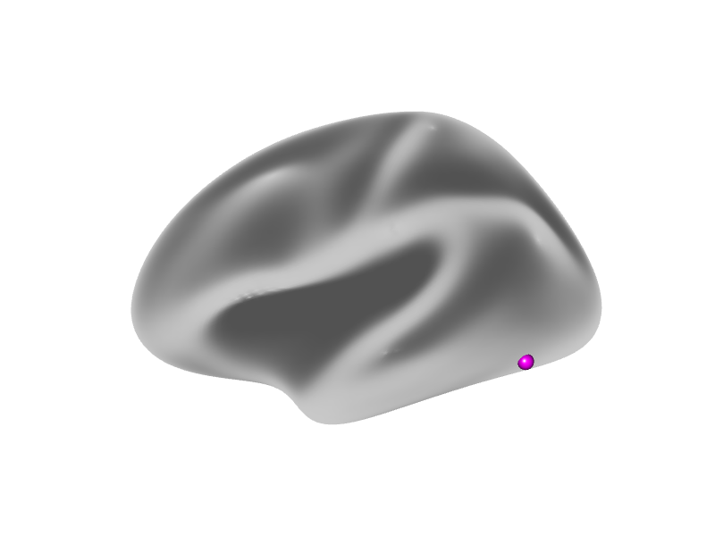
Plotting Other NeuroSurface Objects

The plot() method also works for other classes like NeuroSurface, LabeledNeuroSurface, and ColorMappedNeuroSurface. These objects already contain data and potentially color mapping information. The plot method extracts this information and passes the appropriate arguments (like vals, cmap, irange, thresh, vert_clrs) to the underlying view_surface function.

# Create a NeuroSurface object with the random data
nsurf <- NeuroSurface(white_lh_display, indices = 1:length(random_vals_display), data = random_vals_display)

# Plot the NeuroSurface - uses data stored within the object
# We can still override or add parameters like cmap, irange, thresh, alpha etc.
render_surface(geometry(nsurf), vals = values(nsurf), cmap = heat.colors(128),
               irange = c(-2.5, 2.5), viewpoint = "lateral")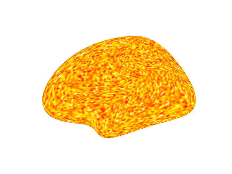
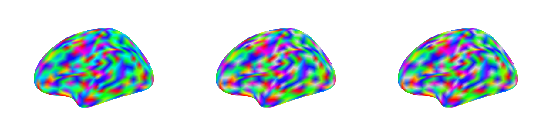
#> file:////private/var/folders/9h/nkjq6vss7mqdl4ck7q1hd8ph0000gp/T/Rtmp8JJqZZ/file1688a7cc18093.html screenshot completed

Showing an activation map overlaid on a surface mesh

We will plot surface in a row of 3. We generate a set of random values and then smooth those values along the surface to approximate a realistic activation pattern.

In the first column we display all the values in the map. Next we threshold all values between (-2,2). In the last panel we additionally add a cluster size threshold of 30 nodes.

vals <- rnorm(length(nodes(white_lh_base)))
surf <- NeuroSurface(white_lh_base, indices = 1:length(vals), data = vals)
ssurf <- smooth(surf)

# Generate proper figure paths
.render_counter$n <- .render_counter$n + 1
act_file1 <- knitr::fig_path(paste0("-actmap-", .render_counter$n, ".png"))
.render_counter$n <- .render_counter$n + 1
act_file2 <- knitr::fig_path(paste0("-actmap-", .render_counter$n, ".png"))
.render_counter$n <- .render_counter$n + 1
act_file3 <- knitr::fig_path(paste0("-actmap-", .render_counter$n, ".png"))
dir.create(dirname(act_file1), recursive = TRUE, showWarnings = FALSE)

# Panel 1: All values
img1 <- try(snapshot_surface(geometry(ssurf), file = act_file1, vals = values(ssurf), cmap = rainbow(100),
                              irange = c(-2, 2), width = 600, height = 450), silent = TRUE)
#> file:////private/var/folders/9h/nkjq6vss7mqdl4ck7q1hd8ph0000gp/T/Rtmp8JJqZZ/file1688a29c1e627.html screenshot completed

# Panel 2: Thresholded (values between -0.2 and 0.2 transparent)
comp <- conn_comp(ssurf, threshold = c(-0.2, 0.2))
img2 <- try(snapshot_surface(geometry(ssurf), file = act_file2, vals = values(ssurf), cmap = rainbow(100),
                              irange = c(-2, 2), thresh = c(-0.2, 0.2), width = 600, height = 450), silent = TRUE)
#> file:////private/var/folders/9h/nkjq6vss7mqdl4ck7q1hd8ph0000gp/T/Rtmp8JJqZZ/file1688a78ed1fdb.html screenshot completed

# Panel 3: Cluster thresholded (minimum cluster size of 30)
csurf <- cluster_threshold(ssurf, size = 30, threshold = c(-0.2, 0.2))
img3 <- try(snapshot_surface(geometry(csurf), file = act_file3, vals = values(csurf), cmap = rainbow(100),
                              irange = c(-2, 2), thresh = c(-0.2, 0.2), width = 600, height = 450), silent = TRUE)
#> file:////private/var/folders/9h/nkjq6vss7mqdl4ck7q1hd8ph0000gp/T/Rtmp8JJqZZ/file1688a17c6a0e3.html screenshot completed

# Check if all snapshots succeeded
valid <- sapply(list(img1, img2, img3), function(p) !inherits(p, "try-error") && length(p) > 0 && file.exists(p))

if (all(valid)) {
  knitr::include_graphics(c(img1, img2, img3))
} else {
  # Fallback to rglwidget
  rgl::open3d()
  rgl::mfrow3d(1, 3, byrow = TRUE)
  view_surface(geometry(ssurf), vals = values(ssurf), cmap = rainbow(100),
               irange = c(-2, 2), new_window = FALSE)
  rgl::next3d()
  view_surface(geometry(ssurf), vals = values(ssurf), cmap = rainbow(100),
               irange = c(-2, 2), thresh = c(-0.2, 0.2), new_window = FALSE)
  rgl::next3d()
  view_surface(geometry(csurf), vals = values(csurf), cmap = rainbow(100),
               irange = c(-2, 2), thresh = c(-0.2, 0.2), new_window = FALSE)
  rgl::rglwidget()
}

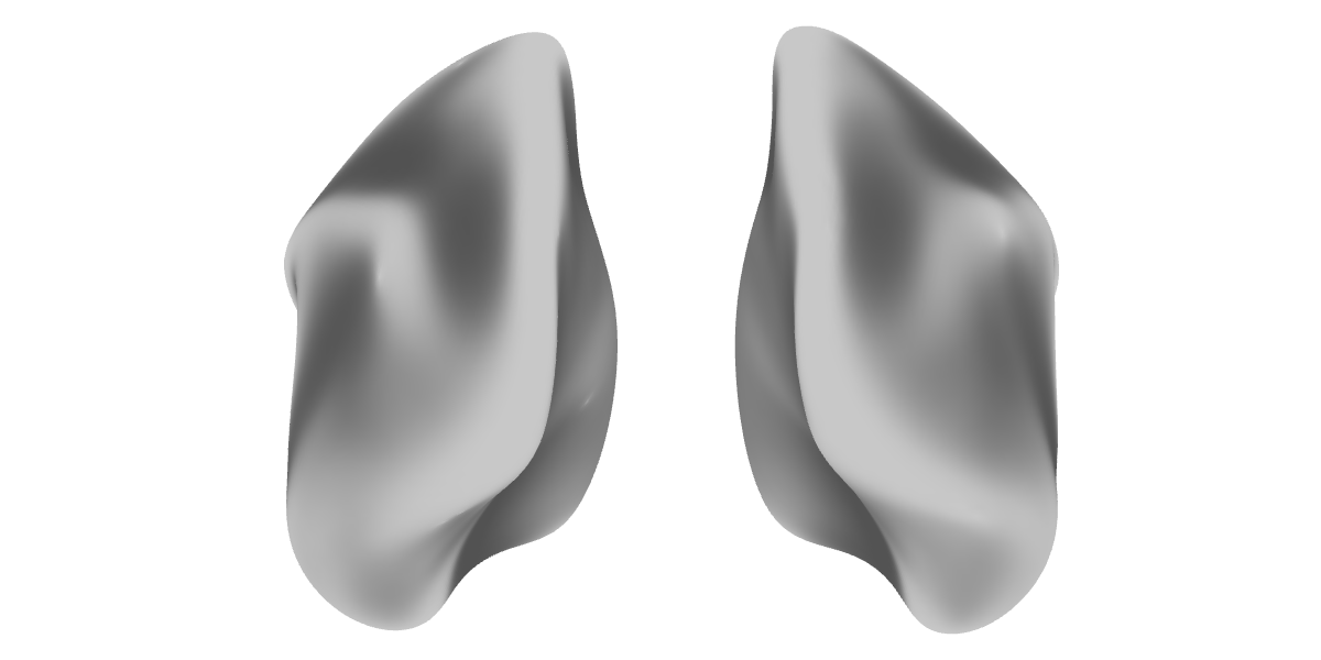
Showing two hemispheres in same scene

# Two hemispheres shown from posterior viewpoint
.render_counter$n <- .render_counter$n + 1
posterior_file <- knitr::fig_path(paste0("-posterior-", .render_counter$n, ".png"))
dir.create(dirname(posterior_file), recursive = TRUE, showWarnings = FALSE)

img_path <- try({
  file <- posterior_file
  rgl::open3d()
  rgl::par3d(windowRect = c(0, 0, 1200, 600))
  rgl::bg3d(color = "white")

  view_surface(white_lh_display, bgcol = curv_cols(curv_lh_display),
               viewpoint = "posterior", new_window = FALSE)
  view_surface(white_rh_smooth, bgcol = curv_cols(curv_rh),
               viewpoint = "posterior", new_window = FALSE, offset = c(100, 0, 0))

  if (rgl::rgl.useNULL() && requireNamespace("webshot2", quietly = TRUE)) {
    rgl::snapshot3d(file, webshot = TRUE)
  } else {
    rgl::rgl.snapshot(file)
  }
  rgl::close3d()
  file
}, silent = TRUE)
#> Warning in min(x): no non-missing arguments to min; returning Inf
#> Warning in max(x): no non-missing arguments to max; returning -Inf
#> Warning in min(x): no non-missing arguments to min; returning Inf
#> Warning in max(x): no non-missing arguments to max; returning -Inf
#> file:////private/var/folders/9h/nkjq6vss7mqdl4ck7q1hd8ph0000gp/T/Rtmp8JJqZZ/file1688a4fb2fb2a.html screenshot completed

if (!inherits(img_path, "try-error") && file.exists(img_path)) {
  knitr::include_graphics(img_path)
} else {
  # Fallback to rglwidget
  rgl::open3d()
  view_surface(white_lh_display, bgcol = curv_cols(curv_lh_display),
               viewpoint = "posterior", new_window = FALSE)
  view_surface(white_rh_smooth, bgcol = curv_cols(curv_rh),
               viewpoint = "posterior", new_window = FALSE, offset = c(100, 0, 0))
  rgl::rglwidget()
}

Next Steps

For interactive 3D visualization with surfwidget(), see vignette("interactive-surfaces").

For publication-quality multi-view figures, see vignette("surfplot-style-figures").

Bradley Buchsbaum

2026-02-03