Diagnostic plots for mixeff fits

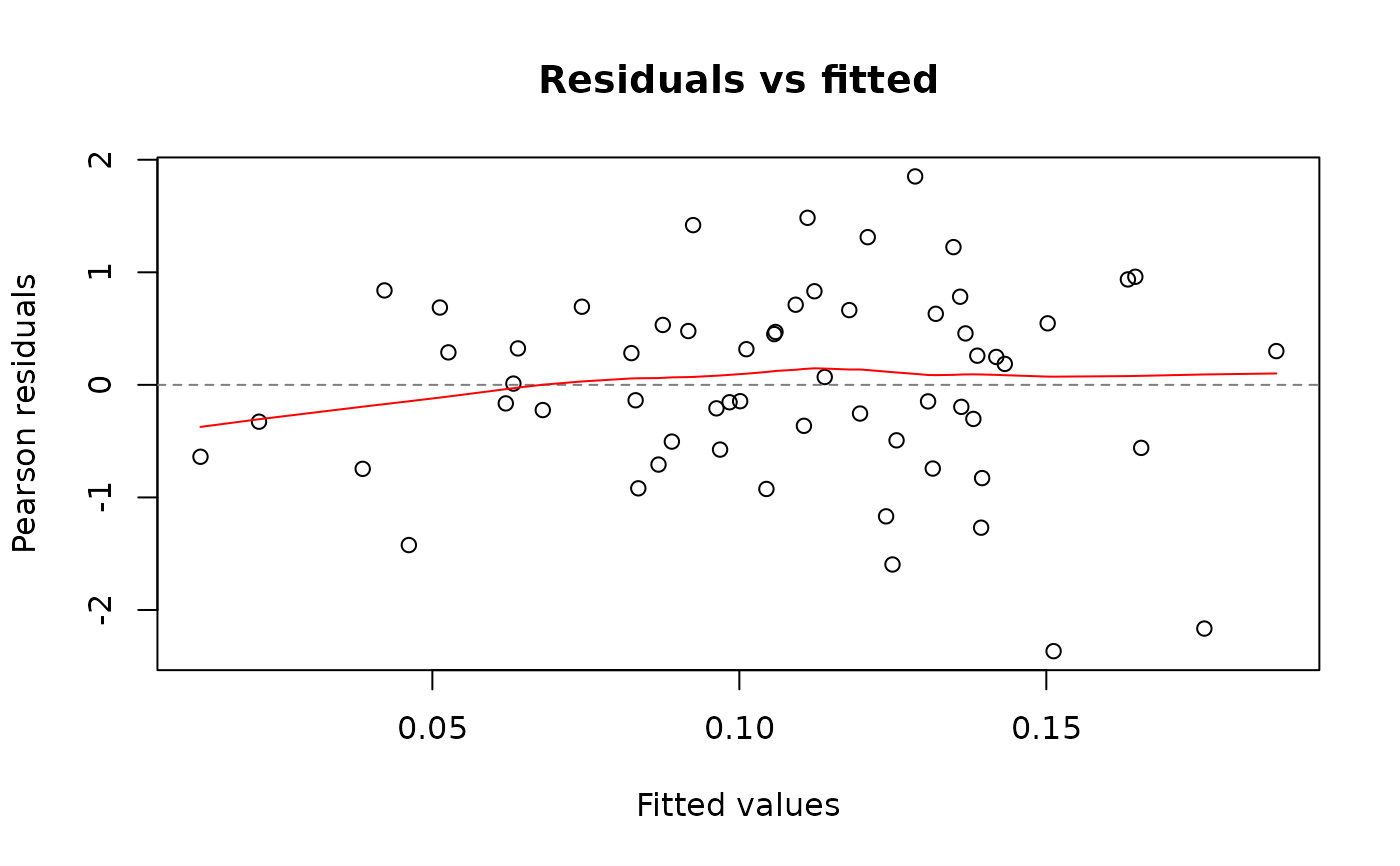
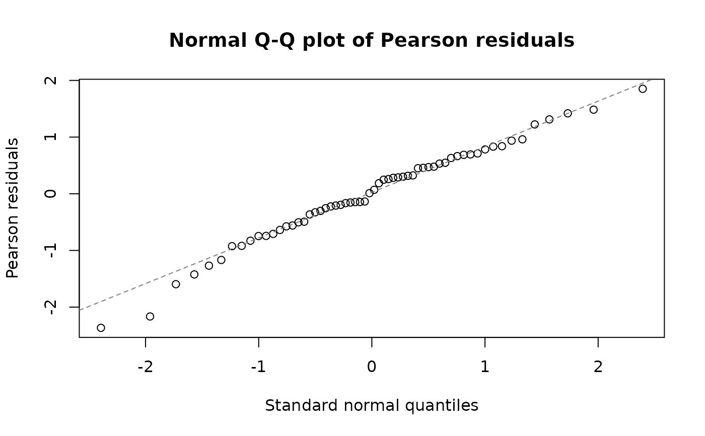
plot() on a fitted model draws Pearson residuals against fitted values, the default diagnostic of lme4's plot.merMod(), using base graphics. which = 2 draws a normal quantile-quantile plot of the Pearson residuals instead (also available as qqnorm(fit)), and which = 3 the scale-location plot (sqrt(|r|) against fitted values).

Usage

# S3 method for class 'mm_lmm'
plot(
  x,
  which = 1L,
  smooth = TRUE,
  ask = length(which) > 1L && grDevices::dev.interactive(),
  main = NULL,
  xlab = NULL,
  ylab = NULL,
  ...
)

# S3 method for class 'mm_glmm'
plot(
  x,
  which = 1L,
  smooth = TRUE,
  ask = length(which) > 1L && grDevices::dev.interactive(),
  main = NULL,
  xlab = NULL,
  ylab = NULL,
  ...
)

# S3 method for class 'mm_lmm'
qqnorm(y, main = NULL, xlab = NULL, ylab = NULL, ...)

# S3 method for class 'mm_glmm'
qqnorm(y, main = NULL, xlab = NULL, ylab = NULL, ...)

Arguments

x, y

A fitted mm_lmm or mm_glmm.

which

Integer vector selecting the plots: 1 residuals vs fitted (default), 2 normal Q-Q of the residuals, 3 scale-location.

smooth

If TRUE (default), add a lowess() smooth to plots 1 and 3.

ask

Ask before each new plot when several are drawn on an interactive device.

main, xlab, ylab

Optional titles overriding the defaults.

...

Further graphical parameters passed to graphics::plot() or stats::qqnorm().

Value

x, invisibly. qqnorm() returns the list from stats::qqnorm() invisibly.

Details

Pearson residuals follow lme4's definition, (y - mu) sqrt(w) / sqrt(V(mu)) with prior weights w and variance function V (V = 1 for an LMM), on the response scale; they are not divided by the residual standard deviation.

See also

plot.mm_ranef() for caterpillar and Q-Q plots of the random effects; hatvalues.mm_lmm() for leverage and Cook's distance.

Examples

set.seed(1)
df <- data.frame(
  y = rnorm(60), x = rnorm(60),
  g = factor(rep(seq_len(10), each = 6))
)
fit <- lmm(y ~ x + (1 | g), df, control = mm_control(verbose = -1))
plot(fit)

plot(fit, which = 2)

qqnorm(fit)