You use a linear mixed model when observations are not independent:
visits within clinics, trials within people, students within classrooms.
The standard R answer is lme4::lmer().
mixeff::lmm() accepts the same formula language —
(1 | group), (x | group),
(1 + x || group), (1 | a/b), crossed blocks —
and the fitted object answers to the common generics:
fixef(), ranef(), VarCorr(),
predict(), summary(), confint(),
anova(), and friends. The supported surface is documented
and closed rather than open-ended:
vignette("mixeff", package = "mixeff") states the contract,
and vignette("lme4-migration", package = "mixeff") gives
the exact verb-and-argument map.
What lmm() adds is that the fitted object carries the
design, the convergence status, and the inference labels with it. You
can audit, summarize, save, and reload without recomputing.
This vignette is the LMM walkthrough: reading a random-effects formula before you fit, fitting, reading the summary, the standard extractors, prediction, and weights — followed by a longer section on what the random-effects spellings themselves mean and the compile-time design help.
The data
The example simulates reaction times (ms) for 18 subjects over ten days of sleep deprivation. Each subject has a different baseline and a different response to continued sleep loss. The data are generated inside this vignette, so the walkthrough runs without an example-data package.
str(sleep)
#> 'data.frame':    180 obs. of  3 variables:
#>  $ Days    : int  0 1 2 3 4 5 6 7 8 9 ...
#>  $ Subject : Factor w/ 18 levels "1","2","3","4",..: 1 1 1 1 1 1 1 1 1 1 ...
#>  $ Reaction: num  224 248 293 300 292 ...
#>  - attr(*, "out.attrs")=List of 2
#>   ..$ dim     : Named int [1:2] 10 18
#>   .. ..- attr(*, "names")= chr [1:2] "Days" "Subject"
#>   ..$ dimnames:List of 2
#>   .. ..$ Days   : chr [1:10] "Days=0" "Days=1" "Days=2" "Days=3" ...
#>   .. ..$ Subject: chr [1:18] "Subject=1" "Subject=2" "Subject=3" "Subject=4" ...
The key structure: Subject appears 10 times in the data
— once per day. Those 10 observations are not independent. They
share the subject’s baseline speed, their individual sensitivity to
sleep loss, and any other between-person trait that we haven’t measured.
If you fit a plain OLS regression, those correlations inflate your Type
I error rate and make standard errors too small.
A mixed model handles this by giving each subject its own intercept and its own slope — their personal baseline and their personal rate of slowing — and then estimating a population distribution over those person-level parameters.
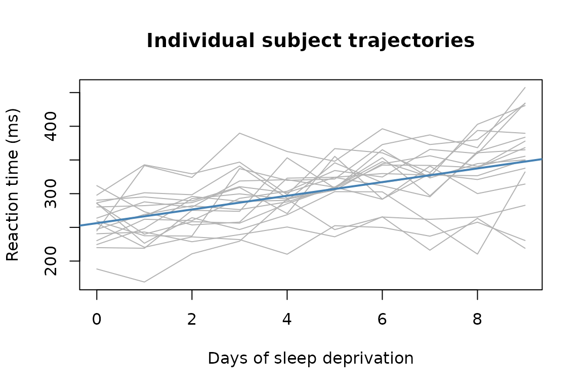
The grey lines are individuals; the blue line is the population average. Subjects vary in their starting point and in how fast they slow down — which is exactly what a random-intercept-and-slope model captures.
Step 1: Read the formula before you fit
Before fitting, compile the model to see what mixeff
understands about your formula. This separates formula interpretation
from optimization; you can catch mis-specified random effects without
paying the cost of a full fit.
spec <- compile_model(Reaction ~ Days + (Days | Subject), sleep)
explain_model(spec)
#> Random effects explanation:
#>   formula: Reaction ~ 1 + Days + (1 + Days | Subject)
#>
#> Random effects:
#>   r0:
#>     wrote:      (Days | Subject)
#>     canonical:  (1 + Days | Subject)
#>     named form: re(group = Subject, intercept = TRUE, slopes = Days, cov = "full")
#>     scope:      `Subject` units differ in baseline and `Days` slope; the model estimates whether these are associated.
#>     covariance: full; theta parameters: 3
#>     support:    sufficient; group levels: 18; min rows/group: 10; median rows/group: 10
#>     variation:  Days=present; intercept=not_assessed
This pre-fit explanation confirms:
- one fixed effect (
Days) plus an intercept, - one random-effects block with a correlated intercept and slope per subject,
- the formula has been canonicalized to the explicit
(1 + Days | Subject)form that the optimizer will receive.
Use audit(spec) when you want the deeper design audit.
Its compact print starts with the audit summary and requested model;
print(audit(spec), full = TRUE) shows the complete upstream
report.
If you had written (1 | Subject) by mistake (random
intercepts only), the explanation would show only one random-effects
column per subject — useful to verify before a long fit. The second half
of this vignette works through the random-effects spellings, canonical
forms, and design diagnostics in detail.
Step 2: Fit
fit <- lmm(Reaction ~ Days + (Days | Subject), sleep)lmm() returns an mm_lmm object. The bundled
Rust engine performs the optimization; lmm() is the R entry
point and result container.
Printing the fit gives the formula, convergence status, likelihood summary, residual scale, and fixed effects.
fit
#> Linear mixed model fit by REML
#> Formula: Reaction ~ Days + (Days | Subject)
#> Fit status: converged_interior
#> Optimizer: trust_bq; iterations: 16; objective: 1715.67
#> nobs: 180, sigma: 23.5052, logLik: -857.837
#> Fixed effects:
#> (Intercept)        Days
#>    256.2570     10.1502
#> Audit verbs: audit(), diagnostics(), inference_table(), model_report()
Step 3: Read the summary
summary(fit, tests = "coefficients")
#> Linear mixed model fit by REML
#> Formula: Reaction ~ Days + (Days | Subject)
#> Fit status: converged_interior
#>
#>  Groups   Name        Std.Dev. Corr
#>  Subject  (Intercept) 25.5476
#>           Days         5.4385  -0.083
#>  Residual             23.5052
#>
#> Fixed effects:
#>              Estimate Std. Error       df   t value  Pr(>|t|)        method
#> (Intercept) 256.25687   6.845681 17.00010 37.433363   < 1e-16 satterthwaite
#> Days         10.15023   1.419585 17.00012  7.150137 1.626e-06 satterthwaite
#>
#> Inference status:
#>         term        method    status reliability
#>  (Intercept) satterthwaite available    moderate
#>         Days satterthwaite available    moderate
#>                             reliability_reason
#>  satterthwaite_finite_difference_approximation
#>  satterthwaite_finite_difference_approximation
#>
#> Notes:
#>   Satterthwaite denominator df computed from analytic vcov_beta Jacobian and finite-difference deviance Hessian over varpar
The summary has four blocks, in print order.
Fit status. Check this line first:
converged_interior is the status every other block of the
summary assumes. When a fit lands somewhere else — a variance component
at zero, a reduced-rank covariance — the status says so and the
available inference methods change with it. What the statuses mean, and
what a boundary does to the rest of the output, is the subject of
vignette("convergence", package = "mixeff").
Variance components.
Subject (Intercept) is the estimated between-subject spread
in baseline reaction time; Subject Days is the estimated
between-subject spread in sensitivity to sleep loss;
correlation is their estimated association. The residual
standard deviation is the within-subject noise left over.
Fixed effects. Estimate is the
population-level coefficient. The Days estimate is the
fitted average change in reaction time per day; the simulation used a
population slope of 10.5 ms per day. The method column
names how each p-value was computed — here satterthwaite, a
finite-sample t test whose df column is on the
scale of the 18 subjects, not the 180 raw rows. Which methods exist,
when each applies, and how to choose among them is covered in
vignette("inference", package = "mixeff").
Inference status. One row per coefficient stating
how much to trust the test: status says whether it was
computed, reliability grades it, and
reliability_reason names the engine’s reason for that grade
— here satterthwaite_finite_difference_approximation, the
standard route for this method. The Rust engine assigns these grades and
reasons; the R side passes them through unchanged. The closed
vocabularies behind these columns are defined in the inference-method
glossary on the package site.
Step 4: Extract components
The lme4-compatible extractors work on mm_lmm
objects.
fixef(fit)
#> (Intercept)        Days
#>   256.25687    10.15023
sigma(fit)
#> [1] 23.50517
logLik(fit)
#> 'log Lik.' -857.8369 (df=6)
VarCorr() reports fitted variance components, and
ranef() returns conditional random effects by grouping
factor.
VarCorr(fit)
#>  Groups   Name        Std.Dev. Corr
#>  Subject  (Intercept) 25.5476
#>           Days         5.4385  -0.083
#>  Residual             23.5052
head(ranef(fit)$Subject)
#>   (Intercept)      Days
#> 1   -8.047859  2.798272
#> 2    4.457929  4.828410
#> 3  -17.179833  4.799052
#> 4   36.246456  4.003062
#> 5   -4.147857  1.625757
#> 6  -23.075999 -8.535978
confint(fit, method = "asymptotic")
#> Confidence intervals:
#>                  2.5 %    97.5 %
#> (Intercept) 242.839579 269.67416
#> Days          7.367891  12.93256
#> method: wald_asymptotic_from_stored_standard_errors
#> status: Wald (asymptotic) intervals from stored standard errors (engine-certified profile intervals: method = "profile")
confint() with method = "asymptotic" gives
Wald intervals. The (Intercept) interval is the population
mean reaction time on Day 0; the Days interval is the range
of plausible slopes. The other interval methods, and when each is
available, are covered in
vignette("inference", package = "mixeff").
Design matrices can be rebuilt from the stored formula and model
frame — including after a save/reload cycle
(vignette("mixeff", package = "mixeff") covers
persistence). getME() rebuilds lme4’s low-level components
(theta, Lambdat, L,
RX, devcomp, …) for code that expects
lme4-style names.
X <- model.matrix(fit, type = "fixed")
Z <- model.matrix(fit, type = "random")

dim(X)
#> [1] 180   2
dim(Z)
#> [1] 180  36
class(Z)
#> [1] "dgCMatrix"
#> attr(,"package")
#> [1] "Matrix"

getME(fit, c("theta", "beta", "cnms"))
#> $theta
#>      Subject.(Intercept) Subject.Days.(Intercept)             Subject.Days
#>               1.08689219              -0.01922107               0.23057417
#>
#> $beta
#> [1] 256.25687  10.15023
#>
#> $cnms
#> $cnms$Subject
#> [1] "(Intercept)" "Days"
For report-ready data-frame tables of the same fit — design summary, random terms, fixed effects — see the reporting article on the package site.
Step 5: Prediction and residuals
For fitted data, predict() returns in-sample fitted
values. Use re.form = NA for the fixed-effect part
only.
prediction_check <- data.frame(
  Reaction = sleep$Reaction,
  fitted = predict(fit),
  fixed_only = predict(fit, re.form = NA),
  residual = residuals(fit)
)
head(prediction_check)
#>   Reaction   fitted fixed_only   residual
#> 1 224.4814 248.2090   256.2569 -23.727602
#> 2 248.2831 261.1575   266.4071 -12.874360
#> 3 292.6939 274.1060   276.5573  18.587938
#> 4 299.7000 287.0545   286.7075  12.645526
#> 5 291.9349 300.0030   296.8578  -8.068130
#> 6 305.1412 312.9515   307.0080  -7.810253
Prediction standard errors and intervals
Population-level prediction standard errors and intervals are
available via re.form = NA (the Wald SE of the fixed-effect
linear predictor):
pop <- predict(fit, re.form = NA, se.fit = TRUE)
head(pop$se.fit)
#>        1        2        3        4        5        6
#> 6.845681 6.651891 6.757396 7.148958 7.783523 8.607515
head(predict(fit, re.form = NA, interval = "confidence"))
#>        fit      lwr      upr
#> 1 256.2569 242.8396 269.6742
#> 2 266.4071 253.3696 279.4446
#> 3 276.5573 263.3131 289.8016
#> 4 286.7075 272.6958 300.7192
#> 5 296.8578 281.6023 312.1132
#> 6 307.0080 290.1376 323.8784
Conditional prediction standard errors (the default,
re.form = NULL) come from the engine’s prediction-variance
payload, which combines the fixed-effect Wald variance with the
random-effect (BLUP) variance and the fixed/random covariance. The
covariance term can be negative, so the conditional SE can come out
smaller than the population SE. Conditional confidence and
prediction intervals come from the same payload.
pred <- predict(fit, se.fit = TRUE)
head(data.frame(population_se = pop$se.fit, conditional_se = pred$se.fit))
#>   population_se conditional_se
#> 1      6.845681      11.757606
#> 2      6.651891      10.086304
#> 3      6.757396       8.665367
#> 4      7.148958       7.635865
#> 5      7.783523       7.168480
#> 6      8.607515       7.370927
head(predict(fit, interval = "confidence"))
#>        fit      lwr      upr
#> 1 248.2090 225.1645 271.2535
#> 2 261.1575 241.3887 280.9263
#> 3 274.1060 257.1222 291.0898
#> 4 287.0545 272.0885 302.0205
#> 5 300.0030 285.9530 314.0530
#> 6 312.9515 298.5048 327.3983
Rows the engine cannot certify — for example an unseen grouping level
predicted with allow.new.levels = TRUE, where there is no
posterior variance for the missing level — return NA with
the engine’s reason in the mm_reason attribute rather than
a fabricated number. That refusal vocabulary is part of the inference
contract (vignette("inference", package = "mixeff")).
Step 6: Case weights
lmm() accepts case weights: one finite, positive value
per row, evaluated in data like the formula variables. A
common use is rows that summarize different numbers of underlying
trials.
sleep$n_trials <- rep(c(1, 2), length.out = nrow(sleep))

fit_w <- lmm(Reaction ~ Days + (Days | Subject), sleep,
             weights = n_trials,
             control = mm_control(verbose = -1))
fixef(fit_w)
#> (Intercept)        Days
#>   255.72882    10.30777
head(fit_w$weights)
#> [1] 1 2 1 2 1 2
The weights are stored on the fit and reused by refit()
and the inference routines. Invalid weights — wrong length, negative, or
non-finite — are refused with a typed mm_data_error rather
than silently recycled.
For contrasts, term tests, marginal means, and model comparisons on a
fit like this one, continue with
vignette("inference", package = "mixeff"). The rest of this
vignette turns to the random-effects formulas themselves.
Random-effects formulas in depth
Random-effects formulas are compact, and compactness hides
assumptions. Seven characters — (x | g) — commit the
analyst to a specific covariance structure, a specific number of free
parameters, and a specific identification claim about what the data can
support. Two formulas that differ by a single character —
|| for |, say — fit different models.
mixeff shares the formula language with
lme4, so the notation you already read transfers directly.
What it adds is a way to read the formula before the optimizer
runs: the named form of every random term, the plain-language scope, the
parameter count, and the design facts that support or refuse the formula
on this particular data.
The goal of this section is not to pick a model for you. It is to show what the model you wrote can and cannot express, and to make the difference between nearby spellings legible.
We use a second small repeated-measures dataset with one row per subject per time point.
head(study)
#>   subject time        dose          x          z    score         y hit
#> 1       1    1 -0.59103110  1.2023289  0.9569158 2.085034 0.6487779   1
#> 2       2    1  0.02659437 -1.0278654  0.6381313 2.469368 0.6684857   1
#> 3       3    1 -1.51655310  0.9382700  1.7919729 2.546363 1.9076263   1
#> 4       4    1 -1.36265335 -0.5431547  1.1717927 1.768118 0.2011020   0
#> 5       5    1  1.17848916  0.5130951  1.4401183 2.062263 0.9445929   1
#> 6       6    1 -0.93415132 -0.3525909 -1.3062800 3.130125 0.7523965   1
What does (1 | subject) say?
A random intercept is the simplest random-effects structure: subjects
may differ in average score, but the fixed time effect is
the same across subjects. It is often the right choice, and it is always
a reasonable starting point. explain_model() spells out
what the model assumes and reports that no random slopes were added.
intercept_only <- compile_model(score ~ time + (1 | subject), study)
explain_model(intercept_only)
#> Random effects explanation:
#>   formula: score ~ 1 + time + (1 | subject)
#>
#> Random effects:
#>   r0:
#>     wrote:      (1 | subject)
#>     canonical:  (1 | subject)
#>     named form: re(group = subject, intercept = TRUE, slopes = NULL, cov = "scalar")
#>     scope:      `subject` units may differ in average outcome.
#>     covariance: scalar; theta parameters: 1
#>     support:    sufficient; group levels: 30; min rows/group: 5; median rows/group: 5
#>     variation:  intercept=not_assessed
#>
#> Design notes:
#>   scope_note: `time` varies within `subject`, so a `subject`-level slope is structurally possible
Each random-effects card has two header lines worth pausing on.
wrote: is the term as you typed it. canonical:
is what the parser hands downstream — what the optimizer, the audit, and
the inference contract will actually see. They are identical here
because (1 | subject) is already in canonical form —
nothing was rewritten. The two diverge for more elaborate formulas.
(1 | clinic/site) is rewritten as
(1 | clinic) + (1 | clinic:site); implicit intercepts are
made explicit; double-bar shorthand expands to its split-block form. The
canonical: line is where you read off the model the engine
will actually fit.
The remaining lines decode the term further. named form:
restates it as a function call that names the grouping factor, the
intercept, the slopes (if any), and the covariance family.
scope: is a plain-language sentence.
covariance and support report parameter cost
and design sufficiency.
The Design notes: section at the bottom records facts
about the data that the fitted formula did not use. Here
time varies within each subject, so a subject-level
time slope is structurally possible. That is reported as a
note, not a correction: whether to add (time | subject) is
a scientific question about whether subjects plausibly differ in their
time slopes, not a mechanical one about what the package
can do.
What changes when you add a random slope?
(1 + time | subject) requests a two-dimensional random
effect for each subject: one baseline coefficient and one
time coefficient, with a fitted covariance between
them.
full <- compile_model(score ~ time + (1 + time | subject), study)
explain_model(full)
#> Random effects explanation:
#>   formula: score ~ 1 + time + (1 + time | subject)
#>
#> Random effects:
#>   r0:
#>     wrote:      (1 + time | subject)
#>     canonical:  (1 + time | subject)
#>     named form: re(group = subject, intercept = TRUE, slopes = time, cov = "full")
#>     scope:      `subject` units differ in baseline and `time` slope; the model estimates whether these are associated.
#>     covariance: full; theta parameters: 3
#>     support:    sufficient; group levels: 30; min rows/group: 5; median rows/group: 5
#>     variation:  intercept=not_assessed; time=present
After fitting, parameterization() shows the optimizer’s
internal coordinates: the vector θ the engine actually searched
over, and where each entry sits in the random-effects covariance
factor.
full_fit <- lmm(
  score ~ time + (1 + time | subject),
  study,
  control = mm_control(verbose = -1)
)
parameterization(full_fit)$table[, c("theta_name", "theta_value", "lambda_value")]
#>                     theta_name theta_value lambda_value
#> 1 theta[0:intercept,intercept]   1.0706638    1.0706638
#> 2      theta[0:time,intercept]   0.1222134    0.1222134
#> 3           theta[0:time,time]   0.5466992    0.5466992
What θ is, why the engine optimizes it rather than the covariance
matrix directly, and how boundary fits are read off this table are
covered in vignette("convergence", package = "mixeff").
What do split blocks and || mean?
The formula (1 | subject) + (0 + time | subject) uses
two separate blocks for the same grouping factor. That fixes the
intercept-slope covariance to zero.
split_blocks <- compile_model(
  score ~ time + (1 | subject) + (0 + time | subject),
  study
)
explain_model(split_blocks)
#> Random effects explanation:
#>   formula: score ~ 1 + time + (1 | subject) + (0 + time | subject)
#>
#> Random effects:
#>   subject has 2 separate random-effect blocks.
#>   r0:
#>     wrote:      (1 | subject)
#>     canonical:  (1 | subject)
#>     named form: re(group = subject, intercept = TRUE, slopes = NULL, cov = "scalar")
#>     scope:      `subject` units may differ in average outcome.
#>     covariance: scalar; theta parameters: 1
#>     support:    sufficient; group levels: 30; min rows/group: 5; median rows/group: 5
#>     variation:  intercept=not_assessed
#>   r1:
#>     wrote:      (0 + time | subject)
#>     canonical:  (0 + time | subject)
#>     named form: re(group = subject, intercept = FALSE, slopes = time, cov = "scalar")
#>     scope:      `subject` units may differ in their `time` slope.
#>     covariance: scalar; theta parameters: 1
#>     support:    sufficient; group levels: 30; min rows/group: 5; median rows/group: 5
#>     variation:  time=present
#>
#> Relationship between blocks:
#>   r0 <-> r1 (Intercept <-> time): separate random-effect blocks fix the covariance between `Intercept` and `time` to zero.
#>
#> Design notes:
#>   random_slope_without_intercept: random slope term omits a random intercept; this leaves baseline grouping dependence unmodeled unless represented elsewhere
#>   covariance_assumption: the covariance between 'Intercept' and 'time' is fixed at zero by separate random-effect blocks
(1 + time || subject) is a shorthand for the same
split-block model.
double_bar <- compile_model(score ~ time + (1 + time || subject), study)
explain_model(double_bar)
#> Random effects explanation:
#>   formula: score ~ 1 + time + (1 + time || subject)
#>
#> Random effects:
#>   subject has 2 separate random-effect blocks.
#>   r0:
#>     wrote:      (1 + time || subject)
#>     canonical:  (1 | subject)
#>     named form: re(group = subject, intercept = TRUE, slopes = NULL, cov = "scalar")
#>     scope:      `subject` units may differ in average outcome.
#>     covariance: scalar; theta parameters: 1
#>     support:    sufficient; group levels: 30; min rows/group: 5; median rows/group: 5
#>     variation:  intercept=not_assessed
#>   r1:
#>     wrote:      (1 + time || subject)
#>     canonical:  (0 + time | subject)
#>     named form: re(group = subject, intercept = FALSE, slopes = time, cov = "scalar")
#>     scope:      `subject` units may differ in their `time` slope.
#>     covariance: scalar; theta parameters: 1
#>     support:    sufficient; group levels: 30; min rows/group: 5; median rows/group: 5
#>     variation:  time=present
#>
#> Relationship between blocks:
#>   r0 <-> r1 (Intercept <-> time): double-bar syntax fixes the covariance between `Intercept` and `time` to zero.
#>
#> Design notes:
#>   covariance_assumption: the covariance between 'Intercept' and 'time' is fixed at zero by || syntax
A factor inside || expands as in lme4:
(1 + x + f || g) is
(1 | g) + (0 + x | g) + (0 + f | g), so the factor keeps
its own correlated block. To fix every covariance at zero, factor
columns included (MixedModels.jl’s zerocorr()), write
diag(1 + x + f | g);
vignette("lme4-migration", package = "mixeff") has the
details.
Nested and crossed grouping
Nesting is written with / and expands mechanically:
(1 | clinic/ward) means one intercept block per clinic plus
one per ward-within-clinic. Crossed factors are simply two blocks —
(1 | subject) + (1 | item) — and nothing is rewritten,
because that spelling is already canonical.
mm_parse_formula() shows the canonical string for any
formula without touching data:
mm_parse_formula("rt ~ days + (1 | subject/task)")
#> [1] "rt ~ 1 + days + (1 | subject) + (1 | subject:task)"
mm_parse_formula("rt ~ days + (1 | subject) + (1 | item)")
#> [1] "rt ~ 1 + days + (1 | subject) + (1 | item)"
mm_parse_formula("rt ~ days + (1 + days || subject)")
#> [1] "rt ~ 1 + days + (1 + days || subject)"
The explain_model() cards agree with these
canonicalizations — they show the model the engine actually fits — with
one display difference: mm_parse_formula() keeps a
|| term as written, while the cards additionally show it as
the split blocks the engine fits.
What are the three kinds of help?
The compile-time diagnostics separate three situations that are often mixed together in ordinary model output.
First, a structural impossibility: a requested random slope cannot be
estimated if that variable does not vary within the group. Here
dose is constant within each subject.
impossible <- compile_model(score ~ dose + (1 + dose | subject), between_study)
explain_model(impossible)
#> Random effects explanation:
#>   formula: score ~ 1 + dose + (1 + dose | subject)
#>
#> Random effects:
#>   r0:
#>     wrote:      (1 + dose | subject)
#>     canonical:  (1 + dose | subject)
#>     named form: re(group = subject, intercept = TRUE, slopes = dose, cov = "full")
#>     scope:      `subject` units differ in baseline and `dose` slope; the model estimates whether these are associated.
#>     covariance: full; theta parameters: 3
#>     support:    sufficient; group levels: 30; min rows/group: 5; median rows/group: 5
#>     variation:  dose=absent; intercept=not_assessed
#>
#> Possible repairs, not applied automatically:
#>   1. structural_refusal: `dose` does not vary within `subject`, so a `subject`-level `dose` slope cannot be estimated from this design.
Second, low information budget: a requested full covariance can be estimable in principle while still having little grouping-level support. The package reports the parameter count and observed levels.
low_info <- compile_model(score ~ time + (1 + time | subject), low_study)
diagnostics(low_info)$table[, c("code", "severity", "message")]
#>                  code severity
#> 1 covariance_too_rich  warning
#> 2 covariance_too_rich  warning
#>                                                                              message
#> 1 4 levels are below the v0 full-covariance threshold 15 for 3 covariance parameters
#> 2 4 levels are below the v0 full-covariance threshold 15 for 3 covariance parameters
Third, unmodeled-but-possible: a fixed effect varies within group,
but the random-effects formula does not include the corresponding slope.
This is the quiet design note you saw for
(1 | subject).
diagnostics(intercept_only)$table[, c("code", "severity", "message")]
#>         code severity
#> 1 scope_note     info
#> 2 scope_note     info
#>                                                                               message
#> 1 `time` varies within `subject`, so a `subject`-level slope is structurally possible
#> 2 `time` varies within `subject`, so a `subject`-level slope is structurally possible
How do you inspect nearby formulas?
random_options() is a map of nearby random-effect
spellings for one grouping factor. It marks the current spelling and
reports parameter costs and support facts. It does not rank the
rows.
random_options(intercept_only, group = subject, slope = time)
#> Random-effect options for group: subject
#> Current model:
#>   (1 | subject) <- this is what you wrote
#>   `subject` units may differ in average outcome.
#> Nearby options:
#>   (1 | subject) <- this is what you wrote
#>     varying coefficients: intercept
#>     covariance family:    scalar
#>     theta parameters:     1
#>     design status:        sufficient
#>     plain meaning:        `subject` units may differ in average outcome.
#>   (0 + time | subject)
#>     varying coefficients: time
#>     covariance family:    scalar
#>     theta parameters:     1
#>     design status:        sufficient
#>     plain meaning:        `subject` units may differ in their `time` slope.
#>   (1 | subject) + (0 + time | subject)
#>     varying coefficients: intercept, time
#>     covariance family:    diagonal via separate blocks
#>     theta parameters:     2
#>     design status:        sufficient
#>     plain meaning:        `subject` units may differ in average outcome. `subject` units may differ in their `time` slope. separate random-effect blocks fix the covariance between `Intercept` and `time` to zero.
#>   (1 + time || subject)
#>     varying coefficients: intercept, time
#>     covariance family:    diagonal via separate blocks
#>     theta parameters:     2
#>     design status:        sufficient
#>     plain meaning:        `subject` units may differ in average outcome. `subject` units may differ in their `time` slope. double-bar syntax fixes the covariance between `Intercept` and `time` to zero.
#>   (1 + time | subject)
#>     varying coefficients: intercept, time
#>     covariance family:    full
#>     theta parameters:     3
#>     design status:        sufficient
#>     plain meaning:        `subject` units differ in baseline and `time` slope; the model estimates whether these are associated.
The same information is available as a data frame if you want to build a custom report.
opts <- random_options(intercept_only, group = subject, slope = time)
opts$options[, c("formula", "theta_parameters", "design_status", "current")]
#>                                formula theta_parameters design_status current
#> 1                        (1 | subject)                1    sufficient    TRUE
#> 2                 (0 + time | subject)                1    sufficient   FALSE
#> 3 (1 | subject) + (0 + time | subject)                2    sufficient   FALSE
#> 4                (1 + time || subject)                2    sufficient   FALSE
#> 5                 (1 + time | subject)                3    sufficient   FALSE
Why is there no recommendation row?
mixeff treats formula explanations as an audit problem,
not a model-selection problem. The package reports the current model,
nearby spellings, assumptions, and data-support facts. Choosing among
scientifically different random-effects structures remains part of the
analysis design.
compare_covariance() gives another view of the same
principle: full, diagonal, and scalar covariance families are displayed
side by side, without a preferred row.
compare_covariance(full)
#> Covariance comparison:
#>   r0 / subject / full <- current
#>     basis:            intercept, time
#>     theta parameters: 3
#>     assumes zero:     none
#>     design status:    sufficient
#>   r0 / subject / diagonal
#>     basis:            intercept, time
#>     theta parameters: 2
#>     assumes zero:     off-diagonal covariances
#>     design status:    sufficient
#>   r0 / subject / scalar
#>     basis:            intercept, time
#>     theta parameters: 1
#>     assumes zero:     off-diagonal covariances
#>     design status:    sufficient
Where do fitted-model changes appear?
After fitting, changes() records the journey from the
formula you wrote to the model the engine actually solved. Each row
carries the stage at which something happened, the term it affected, the
status of the change, and three side-by-side renderings: what was
requested, what was effective (after design parsing
and identifiability checks), and what was fitted (after the
optimizer landed). A reduced-rank covariance estimate appears here as a
labeled fact, not an instruction to rewrite the formula (boundary and
reduced-rank outcomes are the subject of
vignette("convergence", package = "mixeff")).
The full row carries a lot of text. We show it in two passes so neither pass wraps awkwardly in the rendered vignette. The first pass names the stage of each change and its status:
| stage | term_id | status | detail |
|---|---|---|---|
| semantic_ir | unchanged | formula display | |
| certificate_time | r0 | full_rank | requested rank 2; fitted rank 2 |
The second pass shows the requested → effective → fitted arc itself, where the three columns are the substance of the report:
| stage | requested | effective | fitted |
|---|---|---|---|
| semantic_ir | score ~ 1 + time + (1 + time | subject) | score ~ 1 + time + (1 + time | subject) | converged_interior |
| certificate_time | intercept, time | intercept, time | full_rank |
Where to go next
| Question | Where |
|---|---|
| What is the supported envelope, and how do fits persist across sessions? | vignette("mixeff", package = "mixeff") |
| How are p-values computed, and which method is right for my fit? | vignette("inference", package = "mixeff") |
| How do I compute marginal means and treatment contrasts? | vignette("inference", package = "mixeff") |
| What do convergence statuses, boundaries, and singular fits mean? | vignette("convergence", package = "mixeff") |
| Can I fit a binomial/Poisson/negative-binomial GLMM? | vignette("glmm", package = "mixeff") |
| I’m coming from lme4 — what’s different? | vignette("lme4-migration", package = "mixeff") |
| How do I write up the results for a paper? | the reporting article on the package site |