Publication-quality activation tables • fmrireport

Overview

cluster_table() is fmrireport’s standalone function for building publication-quality activation tables from any statistical brain volume. It follows COBIDAS reporting guidelines: hierarchical cluster/sub-peak structure, world coordinates, p-values, and optional anatomical labeling.

This vignette walks through creating realistic synthetic activations, detecting clusters, formatting tables, and adding atlas labels.

Creating synthetic activation maps

Real fMRI analyses produce NeuroVol objects from fmrireg or similar packages. For demonstration, we’ll build a synthetic t-statistic volume with Gaussian-shaped activation blobs placed at known locations.

library(fmrireport)
library(neuroim2)
#> Loading required package: Matrix
#> 
#> Attaching package: 'neuroim2'
#> The following object is masked from 'package:base':
#> 
#>     scale

# Define a brain-like volume in MNI-ish space
# 2mm isotropic, 91x109x91 grid, origin at (-90, -126, -72)
sp <- NeuroSpace(c(91, 109, 91),
                 spacing = c(2, 2, 2),
                 origin = c(-90, -126, -72))

# Start with Gaussian noise (simulating a t-stat map under the null)
set.seed(2024)
arr <- array(rnorm(prod(dim(sp))), dim(sp))

Now add Gaussian-shaped activation blobs. We’ll place them at grid coordinates and use a smooth falloff to simulate realistic spatial extent:

# Helper: add a 3D Gaussian blob centered at grid coordinate (cx, cy, cz)
add_gaussian_blob <- function(arr, cx, cy, cz, peak_value, sigma = 4) {
  dims <- dim(arr)
  # Work in a local window for efficiency
  radius <- ceiling(3 * sigma)
  x_range <- max(1, cx - radius):min(dims[1], cx + radius)
  y_range <- max(1, cy - radius):min(dims[2], cy + radius)
  z_range <- max(1, cz - radius):min(dims[3], cz + radius)

  for (xi in x_range) {
    for (yi in y_range) {
      for (zi in z_range) {
        d2 <- (xi - cx)^2 + (yi - cy)^2 + (zi - cz)^2
        arr[xi, yi, zi] <- arr[xi, yi, zi] +
          peak_value * exp(-d2 / (2 * sigma^2))
      }
    }
  }
  arr
}

# Place blobs at grid coordinates that map to known cortical MNI regions.
# With origin=(-90,-126,-72) and spacing=2mm:
#   grid (27,51,65) -> MNI (-38,-26,56) = Left SomMot
#   grid (65,51,65) -> MNI ( 38,-26,56) = Right SomMot
#   grid (46,55,67) -> MNI (  0,-18,62) = Medial motor
#   grid (41,21,39) -> MNI (-10,-86, 4) = Left V1
#   grid (51,21,39) -> MNI ( 10,-86, 4) = Right V1

# Blob 1: Left somatomotor cortex (large, strong activation)
arr <- add_gaussian_blob(arr, cx = 27, cy = 51, cz = 65, peak_value = 8, sigma = 5)

# Blob 2: Right somatomotor cortex (moderate)
arr <- add_gaussian_blob(arr, cx = 65, cy = 51, cz = 65, peak_value = 6, sigma = 4)

# Blob 3: Medial motor / SMA (moderate)
arr <- add_gaussian_blob(arr, cx = 46, cy = 55, cz = 67, peak_value = 5.5, sigma = 3)

# Blob 4: Left primary visual cortex (small, strong)
arr <- add_gaussian_blob(arr, cx = 41, cy = 21, cz = 39, peak_value = 7, sigma = 3)

# Blob 5: Right primary visual cortex (small, moderate)
arr <- add_gaussian_blob(arr, cx = 51, cy = 21, cz = 39, peak_value = 5, sigma = 3)

vol <- NeuroVol(arr, sp)

Let’s visualize the synthetic activation map:

# Show axial slices at the levels where we placed blobs
slices <- c(39, 55, 60, 65, 67)
plot_montage(vol, zlevels = slices, along = 3L,
             cmap = "inferno", ncol = 5L,
             title = "Synthetic t-statistic map")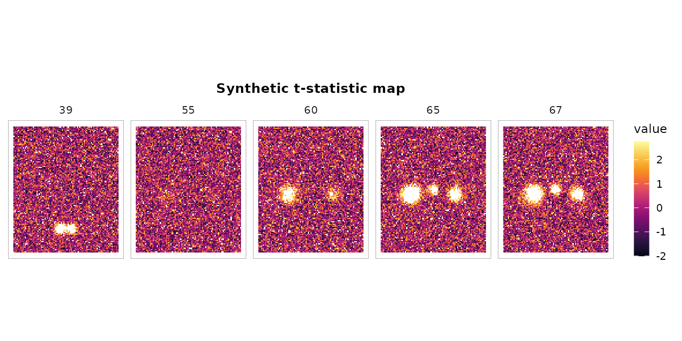

Basic cluster detection

Detect clusters at t > 3.0 with default settings:

ct <- cluster_table(vol,
                    threshold = 3.0,
                    stat_type = "t",
                    df = 100,
                    min_cluster_size = 20)
print(ct)
#> cluster_table: 4 cluster(s)  |  threshold = 3.00 (t)  |  space = Unknown
#> 
#>   Cluster 1  (k = 1623, 12984 mm3)
#>     Peak:   x = -38.0  y = -26.0  z = 52.0  stat = 9.167  p = 6.635e-15
#>       sub-peak 2:  x = -38.0  y = -26.0  z = 54.0  stat = 9.063  p = 1.117e-14
#>       sub-peak 3:  x = -38.0  y = -30.0  z = 54.0  stat = 9.005  p = 1.495e-14
#> 
#>   Cluster 2  (k = 530, 4240 mm3)
#>     Peak:   x = 36.0  y = -28.0  z = 56.0  stat = 8.086  p = 1.485e-12
#>       sub-peak 2:  x = 42.0  y = -24.0  z = 60.0  stat = 7.330  p = 6.078e-11
#>       sub-peak 3:  x = 38.0  y = -28.0  z = 58.0  stat = 7.248  p = 9.031e-11
#> 
#>   Cluster 3  (k = 483, 3864 mm3)
#>     Peak:   x = -10.0  y = -88.0  z = 6.0  stat = 8.573  p = 1.307e-13
#>       sub-peak 2:  x = -10.0  y = -86.0  z = 4.0  stat = 8.439  p = 2.566e-13
#>       sub-peak 3:  x = -12.0  y = -88.0  z = 2.0  stat = 8.410  p = 2.965e-13
#> 
#>   Cluster 4  (k = 187, 1496 mm3)
#>     Peak:   x = -2.0  y = -18.0  z = 60.0  stat = 6.481  p = 3.481e-09
#>       sub-peak 2:  x = 2.0  y = -18.0  z = 62.0  stat = 6.439  p = 4.227e-09
#>       sub-peak 3:  x = -2.0  y = -16.0  z = 60.0  stat = 6.336  p = 6.804e-09

The output shows:

Cluster ID and size (voxels and mm^3)
Peak coordinates in world space (mm)
Peak statistic and p-value
Sub-peaks (local maxima) indented below each cluster

Controlling sub-peak detection

The local_maxima_dist parameter sets the minimum distance (mm) between reported sub-peaks. A larger value gives fewer, more distinct peaks:

# Tight distance: many sub-peaks
ct_tight <- cluster_table(vol, threshold = 3.0, stat_type = "t", df = 100,
                          local_maxima_dist = 8, max_peaks = 5)
cat("Sub-peaks with 8mm distance:\n")
#> Sub-peaks with 8mm distance:
nrow(ct_tight$peaks)
#> [1] 20

# Wide distance: fewer sub-peaks
ct_wide <- cluster_table(vol, threshold = 3.0, stat_type = "t", df = 100,
                         local_maxima_dist = 25, max_peaks = 5)
cat("Sub-peaks with 25mm distance:\n")
#> Sub-peaks with 25mm distance:
nrow(ct_wide$peaks)
#> [1] 20

Sorting options

By default, clusters are sorted by size (descending). You can sort by peak statistic instead:

ct_by_stat <- cluster_table(vol, threshold = 3.0, stat_type = "t", df = 100,
                            sort_by = "peak_stat")
# First cluster has the highest absolute peak stat
ct_by_stat$clusters[, c("cluster_id", "k", "peak_stat")]
#>   cluster_id    k peak_stat
#> 1          1 1623  9.166727
#> 2          3  483  8.573392
#> 3          2  530  8.085848
#> 4          4  187  6.480548

P-value computation

cluster_table() computes voxel-level p-values from the peak statistic and degrees of freedom. Different statistic types are supported:

# t-statistic
ct_t <- cluster_table(vol, threshold = 3.0, stat_type = "t", df = 100)
head(ct_t$clusters[, c("peak_stat", "peak_p")])
#>   peak_stat       peak_p
#> 1  9.166727 6.635204e-15
#> 2  8.085848 1.485288e-12
#> 3  8.573392 1.307328e-13
#> 4  6.480548 3.481219e-09

# z-statistic (provide df to enable p-value computation)
ct_z <- cluster_table(vol, threshold = 3.0, stat_type = "z", df = 1)
head(ct_z$clusters[, c("peak_stat", "peak_p")])
#>   peak_stat       peak_p
#> 1  9.166727 4.876005e-20
#> 2  8.085848 6.173336e-16
#> 3  8.573392 1.004808e-17
#> 4  6.480548 9.138986e-11

# Without df, p-values are NA
ct_nodf <- cluster_table(vol, threshold = 3.0, stat_type = "t", df = NULL)
head(ct_nodf$clusters[, c("peak_stat", "peak_p")])
#>   peak_stat peak_p
#> 1  9.166727     NA
#> 2  8.085848     NA
#> 3  8.573392     NA
#> 4  6.480548     NA

Flat data.frame output

as.data.frame() produces a table where cluster-level rows have all columns populated and sub-peak rows have NA for k and Vol_mm3:

df <- as.data.frame(ct)
df
#>    Cluster    k Vol_mm3   x   y  z     Stat            p Region Hemi
#> 1        1 1623   12984 -38 -26 52 9.166727 6.635204e-15     --   --
#> 2        1   NA      NA -38 -26 54 9.063289 1.117081e-14     --   --
#> 3        1   NA      NA -38 -30 54 9.005398 1.494920e-14     --   --
#> 4        2  530    4240  36 -28 56 8.085848 1.485288e-12     --   --
#> 5        2   NA      NA  42 -24 60 7.330006 6.077715e-11     --   --
#> 6        2   NA      NA  38 -28 58 7.248272 9.030698e-11     --   --
#> 7        3  483    3864 -10 -88  6 8.573392 1.307328e-13     --   --
#> 8        3   NA      NA -10 -86  4 8.438533 2.565961e-13     --   --
#> 9        3   NA      NA -12 -88  2 8.409609 2.964693e-13     --   --
#> 10       4  187    1496  -2 -18 60 6.480548 3.481219e-09     --   --
#> 11       4   NA      NA   2 -18 62 6.438897 4.227018e-09     --   --
#> 12       4   NA      NA  -2 -16 60 6.336318 6.804377e-09     --   --

MNI coordinate column names

When you specify a known coordinate space, column headers adapt:

ct_mni <- cluster_table(vol, threshold = 3.0, stat_type = "t", df = 100,
                        coord_space = "MNI152")
df_mni <- as.data.frame(ct_mni)
names(df_mni)
#>  [1] "Cluster" "k"       "Vol_mm3" "MNI_x"   "MNI_y"   "MNI_z"   "Stat"   
#>  [8] "p"       "Region"  "Hemi"

Formatted tables with tinytable

For inclusion in Quarto/R Markdown reports, format_cluster_tt() produces a tinytable object with an informative caption:

tt <- format_cluster_tt(ct_mni, max_sub_peaks = 2, digits = 2)
tt

Threshold: t = 3 | df = 100 | Space: MNI152
Cluster	k	Vol_mm3	MNI_x	MNI_y	MNI_z	Stat	Region	Hemi
1	1623	12984	-38	-26	52	9.17	--	--
1	NA	NA	-38	-26	54	9.06	--	--
1	NA	NA	-38	-30	54	9.01	--	--
2	530	4240	36	-28	56	8.09	--	--
2	NA	NA	42	-24	60	7.33	--	--
2	NA	NA	38	-28	58	7.25	--	--
3	483	3864	-10	-88	6	8.57	--	--
3	NA	NA	-10	-86	4	8.44	--	--
3	NA	NA	-12	-88	2	8.41	--	--
4	187	1496	-2	-18	60	6.48	--	--
4	NA	NA	2	-18	62	6.44	--	--
4	NA	NA	-2	-16	60	6.34	--	--

Atlas labeling

When you provide an atlas, cluster_table() automatically labels each peak with anatomical region names, hemisphere, and (for parcellation atlases like Schaefer) network assignment.

library(neuroatlas)
#> 
#> Welcome to neuroatlas!
#> To use TemplateFlow features, you'll need to run:
#>   neuroatlas::install_templateflow()
#> This only needs to be done once and will create a persistent environment.
#> For more info, run: neuroatlas::check_templateflow()
#> 
#> Attaching package: 'neuroatlas'
#> The following object is masked from 'package:neuroim2':
#> 
#>     resample

# Load the Schaefer 200-parcel, 7-network atlas
atlas <- get_schaefer_atlas(parcels = "200", networks = "7")
#> downloading: https://raw.githubusercontent.com/ThomasYeoLab/CBIG/master/stable_projects/brain_parcellation/Schaefer2018_LocalGlobal/Parcellations/MNI//freeview_lut/Schaefer2018_200Parcels_7Networks_order.txt

ct_labeled <- cluster_table(vol, threshold = 3.0,
                            stat_type = "t", df = 100,
                            atlas = atlas,
                            coord_space = "MNI152")
print(ct_labeled)
#> cluster_table: 4 cluster(s)  |  threshold = 3.00 (t)  |  space = MNI152  |  atlas = Schaefer-200-7networks
#> 
#>   Cluster 1  (k = 1623, 12984 mm3)
#>     Peak:   [SomMot_10] (left)  MNI x = -38.0  MNI y = -26.0  MNI z = 52.0  stat = 9.167  p = 6.635e-15
#>       sub-peak 2:  [SomMot_10]  MNI x = -38.0  MNI y = -26.0  MNI z = 54.0  stat = 9.063  p = 1.117e-14
#>       sub-peak 3:  MNI x = -38.0  MNI y = -30.0  MNI z = 54.0  stat = 9.005  p = 1.495e-14
#> 
#>   Cluster 2  (k = 530, 4240 mm3)
#>     Peak:   [SomMot_12] (right)  MNI x = 36.0  MNI y = -28.0  MNI z = 56.0  stat = 8.086  p = 1.485e-12
#>       sub-peak 2:  [SomMot_12]  MNI x = 42.0  MNI y = -24.0  MNI z = 60.0  stat = 7.330  p = 6.078e-11
#>       sub-peak 3:  [SomMot_12]  MNI x = 38.0  MNI y = -28.0  MNI z = 58.0  stat = 7.248  p = 9.031e-11
#> 
#>   Cluster 3  (k = 483, 3864 mm3)
#>     Peak:   [Vis_10] (left)  MNI x = -10.0  MNI y = -88.0  MNI z = 6.0  stat = 8.573  p = 1.307e-13
#>       sub-peak 2:  [Vis_7]  MNI x = -10.0  MNI y = -86.0  MNI z = 4.0  stat = 8.439  p = 2.566e-13
#>       sub-peak 3:  [Vis_7]  MNI x = -12.0  MNI y = -88.0  MNI z = 2.0  stat = 8.410  p = 2.965e-13
#> 
#>   Cluster 4  (k = 187, 1496 mm3)
#>     Peak:   [SomMot_15] (left)  MNI x = -2.0  MNI y = -18.0  MNI z = 60.0  stat = 6.481  p = 3.481e-09
#>       sub-peak 2:  [SomMot_18]  MNI x = 2.0  MNI y = -18.0  MNI z = 62.0  stat = 6.439  p = 4.227e-09
#>       sub-peak 3:  [SomMot_15]  MNI x = -2.0  MNI y = -16.0  MNI z = 60.0  stat = 6.336  p = 6.804e-09

The labeled table now includes region name, hemisphere, and network for each peak coordinate:

as.data.frame(ct_labeled)
#>    Cluster    k Vol_mm3 MNI_x MNI_y MNI_z     Stat            p    Region  Hemi
#> 1        1 1623   12984   -38   -26    52 9.166727 6.635204e-15 SomMot_10  left
#> 2        1   NA      NA   -38   -26    54 9.063289 1.117081e-14 SomMot_10  left
#> 3        1   NA      NA   -38   -30    54 9.005398 1.494920e-14        --    --
#> 4        2  530    4240    36   -28    56 8.085848 1.485288e-12 SomMot_12 right
#> 5        2   NA      NA    42   -24    60 7.330006 6.077715e-11 SomMot_12 right
#> 6        2   NA      NA    38   -28    58 7.248272 9.030698e-11 SomMot_12 right
#> 7        3  483    3864   -10   -88     6 8.573392 1.307328e-13    Vis_10  left
#> 8        3   NA      NA   -10   -86     4 8.438533 2.565961e-13     Vis_7  left
#> 9        3   NA      NA   -12   -88     2 8.409609 2.964693e-13     Vis_7  left
#> 10       4  187    1496    -2   -18    60 6.480548 3.481219e-09 SomMot_15  left
#> 11       4   NA      NA     2   -18    62 6.438897 4.227018e-09 SomMot_18 right
#> 12       4   NA      NA    -2   -16    60 6.336318 6.804377e-09 SomMot_15  left

Combining with overlay plots

You can pair the cluster table with a brain overlay visualization:

# Create a thresholded overlay for visualization
arr_thresh <- as.array(vol)
arr_thresh[abs(arr_thresh) < 3.0] <- NA
vol_thresh <- NeuroVol(arr_thresh, sp)

# Create a background volume (uniform gray for this demo)
bg_arr <- array(1000, dim(sp))
bg <- NeuroVol(bg_arr, sp)

plot_overlay(bg, vol_thresh,
             zlevels = c(39, 55, 60, 65),
             along = 3L,
             ov_cmap = "inferno",
             ov_thresh = 0,
             ncol = 4L,
             title = "Thresholded activation (t > 3.0)")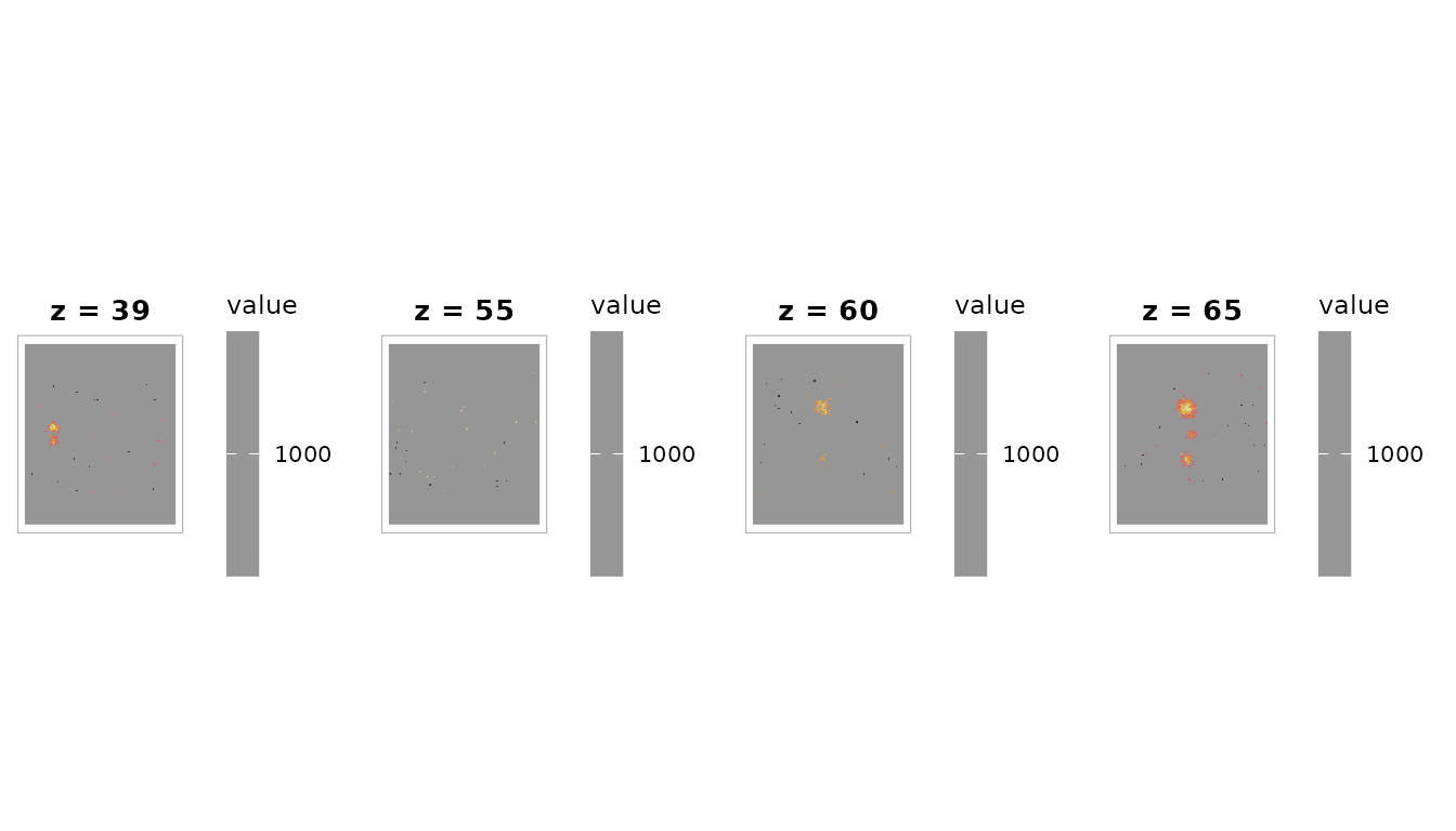

Connectivity options

By default, clusters use 26-connectivity (face, edge, and vertex neighbors). You can switch to more conservative connectivity:

ct_6 <- cluster_table(vol, threshold = 3.0, stat_type = "t", df = 100,
                      connectivity = "6-connect")
ct_26 <- cluster_table(vol, threshold = 3.0, stat_type = "t", df = 100,
                       connectivity = "26-connect")
cat("6-connect clusters:", ct_6$n_clusters, "\n")
#> 6-connect clusters: 4
cat("26-connect clusters:", ct_26$n_clusters, "\n")
#> 26-connect clusters: 4

Stricter connectivity (6-connect) tends to break large clusters into smaller pieces.

Edge cases

The function handles edge cases gracefully:

# No suprathreshold voxels
ct_empty <- cluster_table(vol, threshold = 100)
ct_empty$n_clusters
#> [1] 0
print(ct_empty)
#> cluster_table: 0 clusters (threshold = 100 )

# Very liberal threshold (many small clusters filtered by min_cluster_size)
ct_liberal <- cluster_table(vol, threshold = 1.5, min_cluster_size = 50)
cat("Clusters with k >= 50:", ct_liberal$n_clusters, "\n")
#> Clusters with k >= 50: 20

The cluster_table object

A cluster_table is an S3 list with these elements:

str(ct, max.level = 1)
#> List of 8
#>  $ clusters   :'data.frame': 4 obs. of  12 variables:
#>  $ peaks      :'data.frame': 12 obs. of  11 variables:
#>  $ threshold  : num 3
#>  $ stat_type  : chr "t"
#>  $ df         : num 100
#>  $ n_clusters : int 4
#>  $ coord_space: chr "Unknown"
#>  $ atlas_name : chr NA
#>  - attr(*, "class")= chr "cluster_table"

Element	Type	Description
`clusters`	data.frame	One row per cluster
`peaks`	data.frame	Sub-peaks with rank within cluster
`threshold`	numeric	Detection threshold used
`stat_type`	character	`"t"`, `"z"`, `"F"`, or `"other"`
`df`	numeric	Degrees of freedom (NULL if not provided)
`n_clusters`	integer	Number of clusters
`coord_space`	character	Coordinate space label
`atlas_name`	character	Atlas name or NA

Summary

cluster_table() provides a complete pipeline from statistical volume to publication-ready activation table: 1. Cluster detection via neuroim2::conn_comp() 2. Size filtering 3. World coordinate transformation 4. Sub-peak (local maxima) identification 5. Optional atlas labeling via neuroatlas 6. Parametric p-value computation

Output can be printed to the console, converted to a flat data.frame, or formatted as a tinytable for direct inclusion in reports.