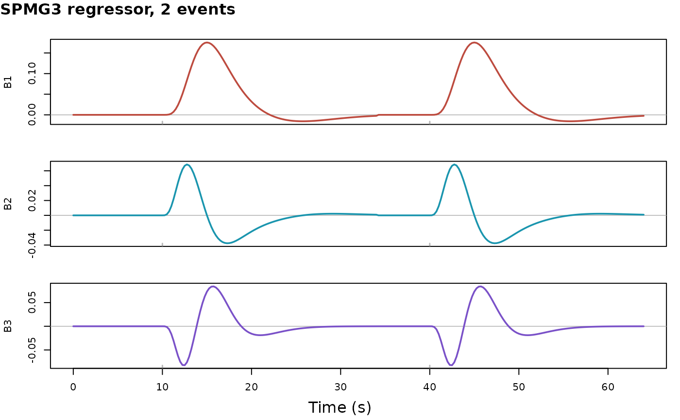
Draws the predicted BOLD time course of a regressor with base graphics. Event onsets are marked with ticks along the time axis. Regressors built from a basis set are drawn one basis function per panel by default.
Arguments
- x
A
Regobject created byregressor().- grid
Numeric vector of time points for evaluation. If NULL (default), uses a grid from 0 to max(onsets) + span with step 0.25 s.
- show_onsets
Logical; if TRUE (default), mark event onsets with ticks on the time axis.
- onset_color
Colour for onset ticks. If NULL (default), a neutral grey.
- onset_alpha
Alpha transparency for onset ticks. Default is 0.5.
- precision
Numeric sampling precision for HRF evaluation. If NULL (default), the grid spacing capped at 0.33 s, so sharp HRF edges are drawn where they occur.
- layout
For multi-basis regressors,
"stack"(default) draws one panel per basis function;"overlay"draws them in a single panel.- ...
Additional arguments passed to
graphics::plot().
See also
plot_regressors() for ggplot2 comparisons of several regressors.
Examples
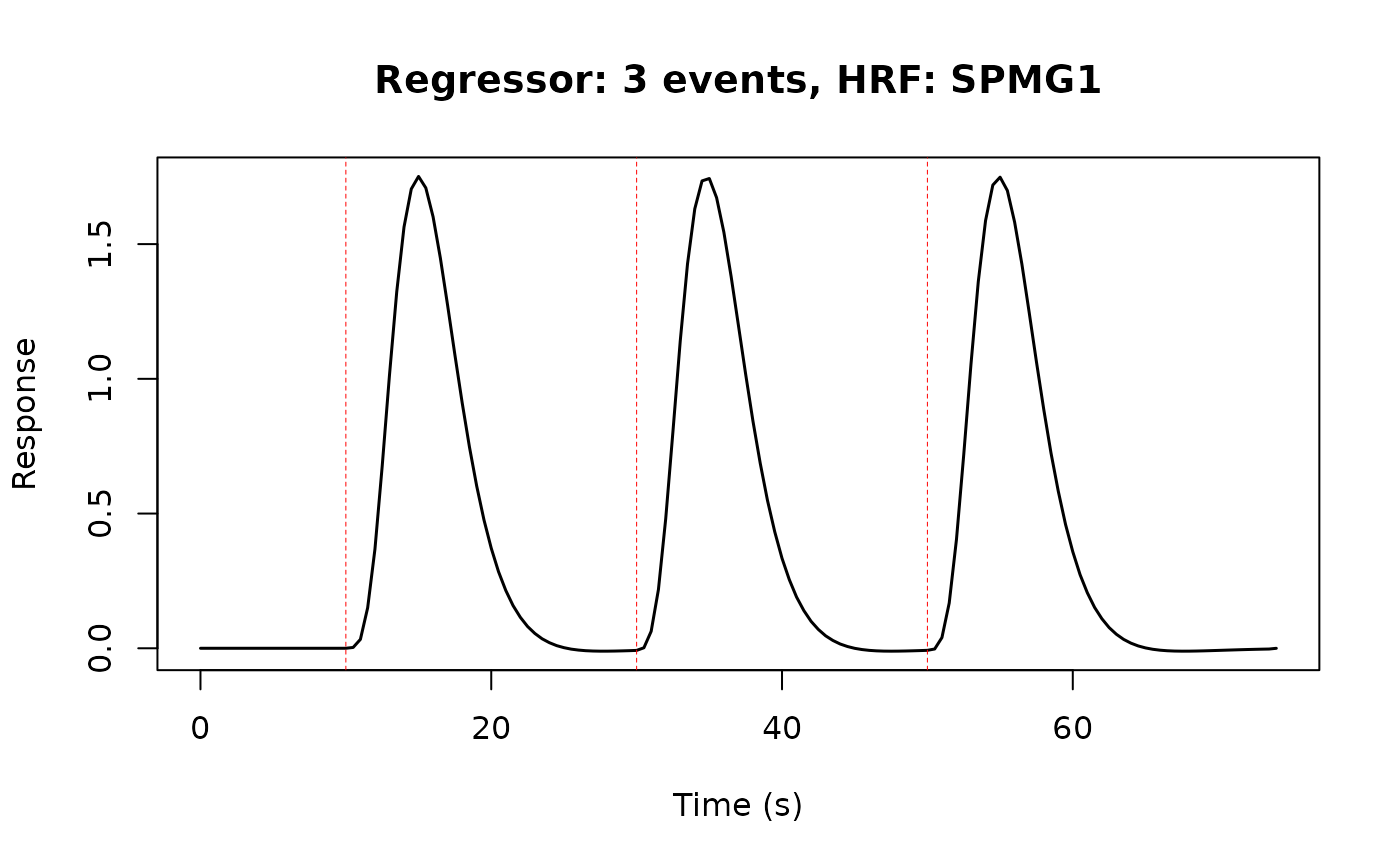
# Create and plot a simple regressor
reg <- regressor(onsets = c(10, 30, 50), hrf = HRF_SPMG1)
plot(reg)
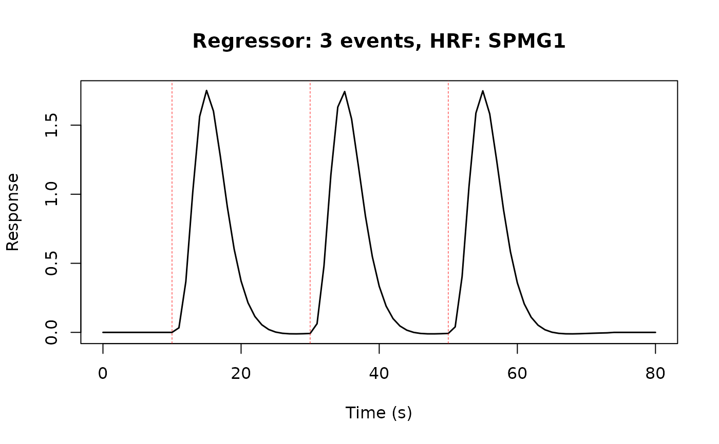
 # Plot with custom time grid
plot(reg, grid = seq(0, 80, by = 1))
# Plot with custom time grid
plot(reg, grid = seq(0, 80, by = 1))
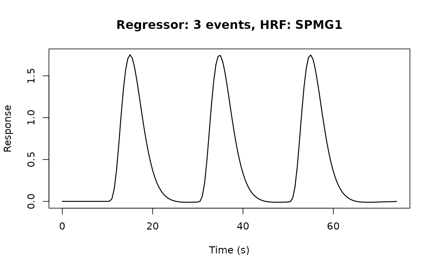
 # Plot without onset markers
plot(reg, show_onsets = FALSE)
# Plot without onset markers
plot(reg, show_onsets = FALSE)
 # A basis-set regressor: one panel per basis function
plot(regressor(c(10, 40), HRF_SPMG3))
# A basis-set regressor: one panel per basis function
plot(regressor(c(10, 40), HRF_SPMG3))