Spatial Neighbor Graphs • adjoin

library(adjoin)
library(Matrix)

When coordinates matter more than features

Many data sets come with known spatial relationships: pixels in an image, voxels in a brain scan, sensors on a grid, measurements at geographic locations. For these data the question “who is my neighbor?” has a physical answer — Euclidean distance in coordinate space — rather than a statistical one derived from feature vectors.

adjoin provides a focused set of functions that build adjacency matrices directly from coordinate matrices. The output is always a sparse Matrix with the same interface as feature-based graphs: adjacency(), laplacian(), and normalization all work the same way.

Your first spatial graph

We will use a 6 × 6 grid throughout this vignette — small enough to visualize, representative of image and brain-imaging data.

coords <- as.matrix(expand.grid(x = 1:6, y = 1:6))   # 36 points, 2 columns
dim(coords)
#> [1] 36  2

spatial_adjacency() connects every point to its nearest spatial neighbors. Two parameters shape the neighborhood:

sigma — the heat kernel bandwidth (larger = broader neighborhood)
nnk — the hard cap on neighbor count (keeps the matrix sparse)

A <- spatial_adjacency(coords, sigma = 1.5, nnk = 8,
                       weight_mode = "heat",
                       include_diagonal = FALSE,
                       normalized = TRUE)
cat("size:", nrow(A), "x", ncol(A),
    "| non-zero entries:", Matrix::nnzero(A), "\n")
#> size: 36 x 36 | non-zero entries: 296
cat("symmetric:", isSymmetric(A), "\n")
#> symmetric: TRUE

Each of the 36 grid points has up to 8 heat-kernel-weighted neighbors within radius sigma × 3 = 4.5 grid units. Normalization symmetrizes the matrix ( $D^{-1/2} A D^{-1/2}$ ) so that edge weights are comparable across nodes with different numbers of neighbors.

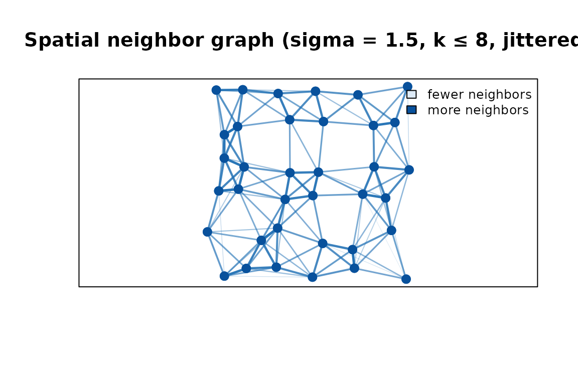
Spatial neighbor graph on a jittered 6 × 6 grid. Thicker, darker lines are higher-weight edges (nearer neighbours); lighter lines are lower-weight (farther neighbours). Point colour encodes degree.

Corner and edge points have fewer neighbors than interior points. Because the coordinates are slightly irregular, edge weights also vary: thicker, darker lines connect closer pairs; faint lines connect pairs near the neighbourhood boundary.

Two weight modes

weight_mode controls how spatial distance is converted to an edge weight.

Mode	Edge weight	Best for
`"heat"`	exp(−d²/2σ²)	Smooth, distance-proportional weights
`"binary"`	1 for every neighbor	Structural analysis, graph spectra

A_heat   <- spatial_adjacency(coords, sigma = 1.5, nnk = 8,
                              weight_mode = "heat",
                              include_diagonal = FALSE, normalized = FALSE,
                              stochastic = FALSE)
A_binary <- spatial_adjacency(coords, sigma = 1.5, nnk = 8,
                              weight_mode = "binary",
                              include_diagonal = FALSE, normalized = FALSE,
                              stochastic = FALSE)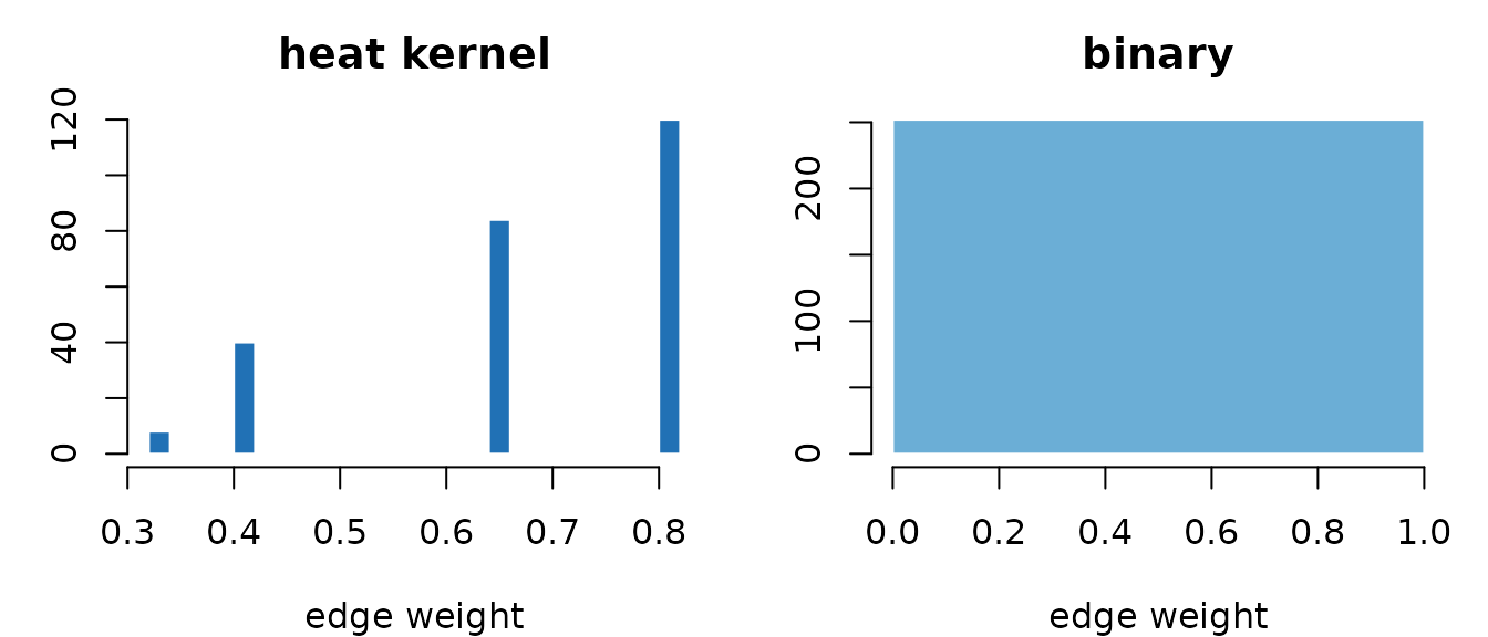

Heat weights decay continuously with distance; binary weights are uniform within the neighborhood radius.

The heat kernel produces a smooth spectrum between 0 and 1; binary produces a single spike at 1. Use "heat" when distance matters, "binary" when only presence of a connection matters.

Effect of sigma on neighborhood size

Increasing sigma extends the neighborhood and softens the weight decay, adding more edges. The nnk cap limits runaway growth.

A_tight <- spatial_adjacency(coords, sigma = 0.8, nnk = 27,
                             weight_mode = "heat",
                             include_diagonal = FALSE, normalized = TRUE)
A_wide  <- spatial_adjacency(coords, sigma = 2.5, nnk = 27,
                             weight_mode = "heat",
                             include_diagonal = FALSE, normalized = TRUE)

c(tight_edges = Matrix::nnzero(A_tight) / 2L,
  wide_edges  = Matrix::nnzero(A_wide)  / 2L)
#> tight_edges  wide_edges 
#>         238         534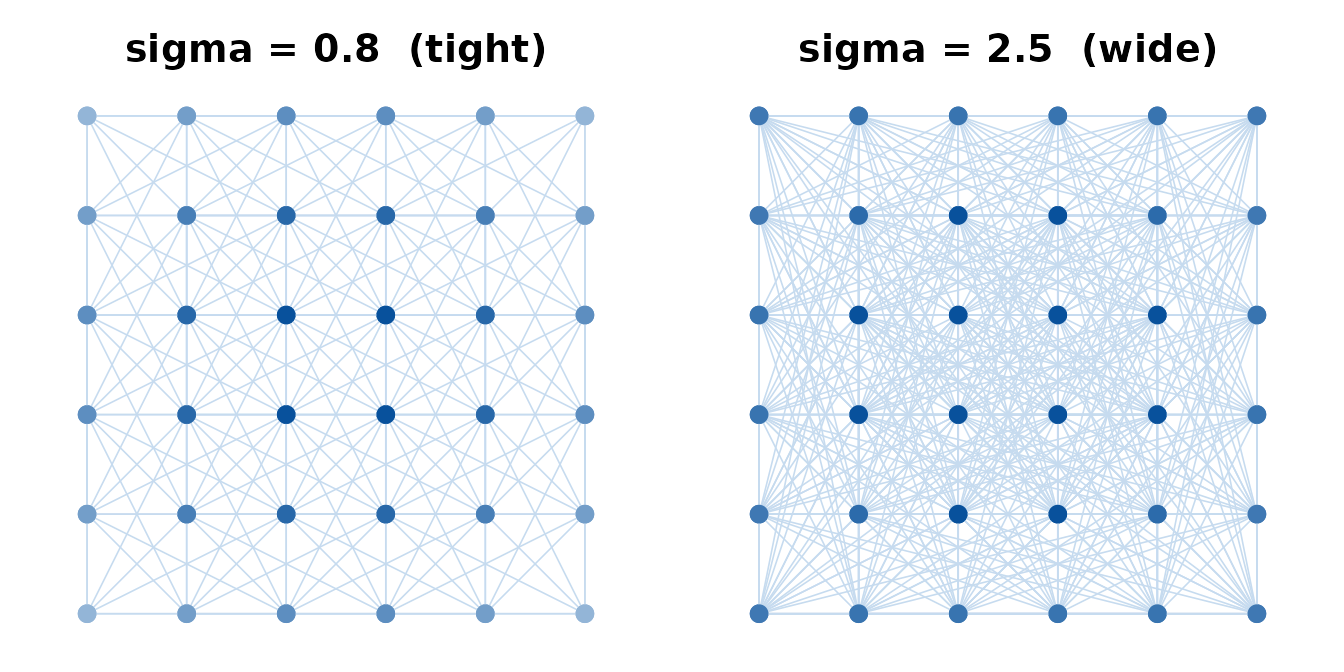

Tight sigma (0.8) leaves corner and edge points with few connections; wide sigma (2.5) connects most points richly.

Spatial smoothing

spatial_smoother() converts a spatial adjacency into a weighted averaging operator. Multiplying any signal vector by S replaces each point’s value with a distance-weighted average of its neighbors.

S <- spatial_smoother(coords, sigma = 1.5, nnk = 8, stochastic = FALSE)

set.seed(42)
signal_raw      <- rnorm(36)
signal_smoothed <- as.numeric(S %*% signal_raw)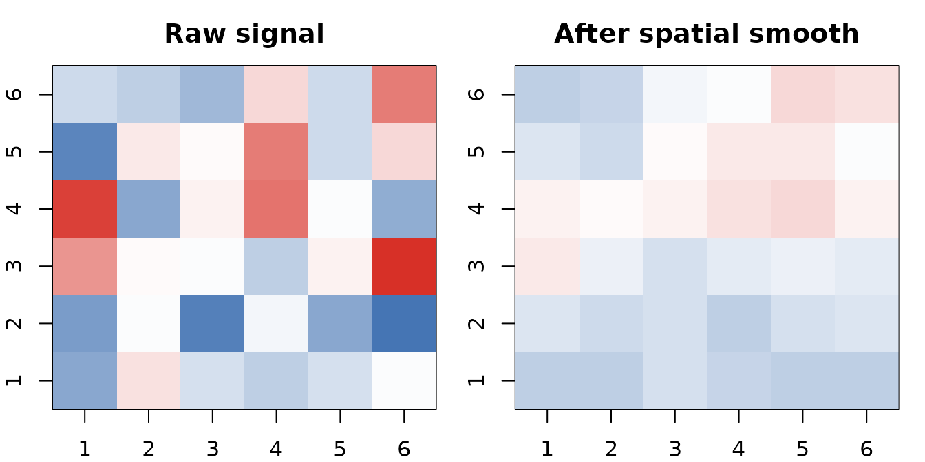

One pass of the spatial smoother turns Gaussian noise (left) into a smoothly varying field (right). The same heat kernel defines both neighbor selection and weight decay.

Set stochastic = TRUE to apply Sinkhorn–Knopp normalization and produce a doubly stochastic smoother (rows and columns sum to 1).

The spatial Laplacian

spatial_laplacian() returns L = D − A, where D is the degree matrix. Multiplying a signal by L measures its local curvature — how much each point deviates from its neighbors.

L <- spatial_laplacian(coords, dthresh = 4.5, nnk = 8,
                       weight_mode = "binary", normalized = FALSE)

# Row sums of a Laplacian are zero by definition
range(round(rowSums(L), 10))
#> [1] 0 0

Use normalized = TRUE for the symmetric form I − D^{−1/2} A D^{−1/2}, which is standard for spectral clustering and graph signal processing.

Combining space and features

When you have both coordinates and feature observations, weighted_spatial_adjacency() blends the two similarity sources. The alpha parameter sweeps from pure spatial weighting to pure feature weighting.

set.seed(42)
features <- matrix(rnorm(36 * 5), nrow = 36, ncol = 5)  # random 5-d features

A_sp  <- weighted_spatial_adjacency(coords, features,
                                    alpha = 0, sigma = 2, nnk = 8)
A_mix <- weighted_spatial_adjacency(coords, features,
                                    alpha = 0.5, sigma = 2, nnk = 8)
A_ft  <- weighted_spatial_adjacency(coords, features,
                                    alpha = 1, sigma = 2, nnk = 8)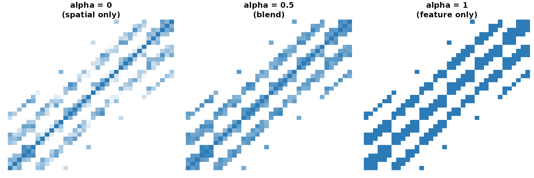

Adjacency heat maps for three alpha values. Spatial-only (left) shows a clean block structure; feature-only (right) looks noisier because the random features carry no spatial signal.

With random features the feature-only matrix is noisy. When features carry genuine spatial signal — say, image intensities — the blend rewards both proximity and similarity.

Bilateral smoothing

bilateral_smoother() is a spatial smoother that down-weights neighbors with very different feature values. This is the classic bilateral filter from image processing: it smooths within regions but preserves sharp edges between them.

# Piecewise-constant signal with a hard boundary at x = 3.5
signal_field <- ifelse(coords[, "x"] <= 3, -1, 1) + rnorm(36, sd = 0.2)
feature_mat  <- matrix(signal_field, ncol = 1)

B                <- bilateral_smoother(coords, feature_mat,
                                       nnk = 8, s_sigma = 1.5, f_sigma = 0.5)
signal_bilateral <- as.numeric(B %*% signal_field)
signal_spatial   <- as.numeric(S %*% signal_field)   # plain spatial smoother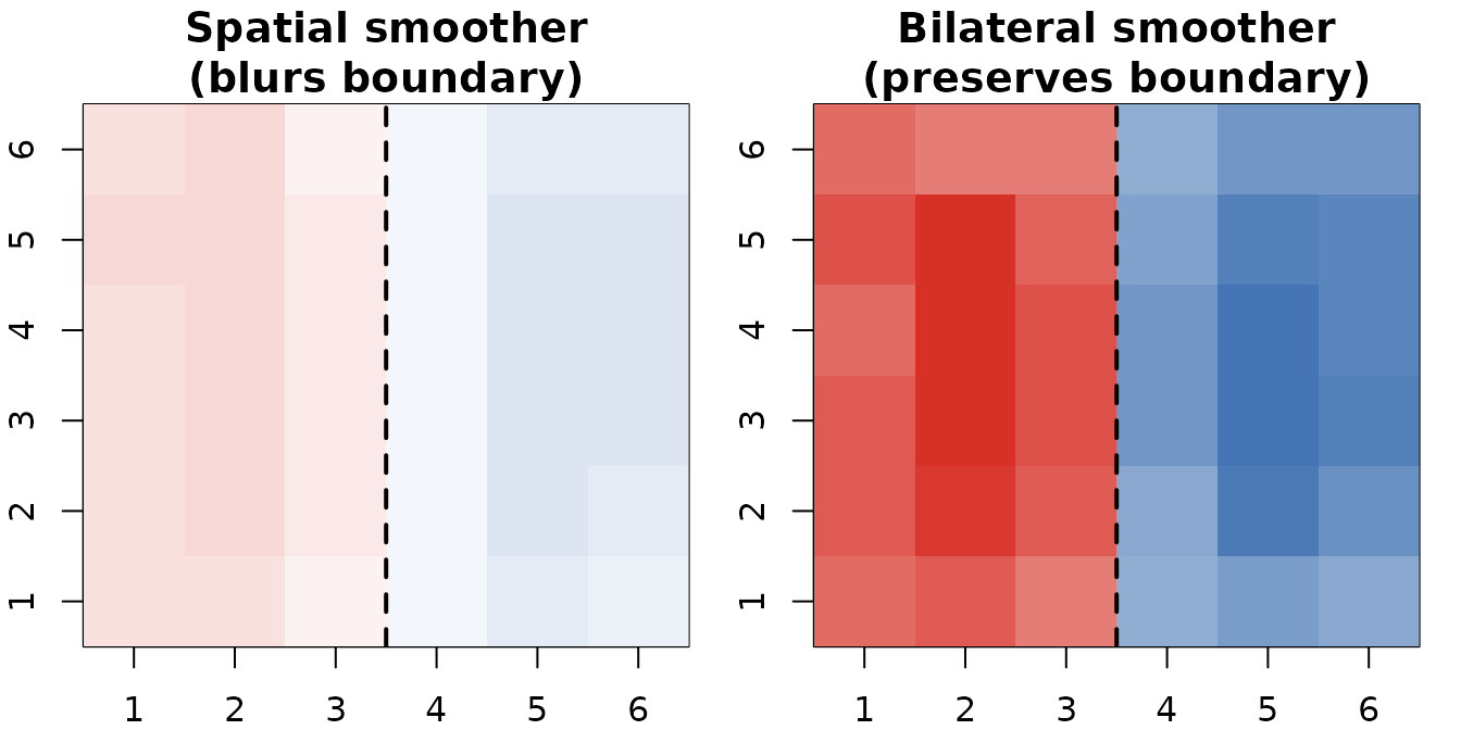

Bilateral smoother (right) preserves the hard boundary between the two signal regions; a plain spatial smoother (left) blurs across it.

The f_sigma parameter controls how sensitive the filter is to feature differences: smaller values enforce stricter edge preservation.

Multi-block spatial constraints

spatial_constraints() handles the case where the same spatial layout appears across multiple blocks — for example, the same brain or image grid measured across subjects or sessions. It builds a combined constraint matrix encoding:

Within-block connections: heat-kernel spatial similarity within each block
Between-block connections: correspondence between matching locations across blocks

The shrinkage_factor balances these two: 0 = all within-block, 1 = all between-block.

coords_small <- as.matrix(expand.grid(x = 1:4, y = 1:4))  # 16-point grid

# Pass a list with one entry per block (same grid repeated for two subjects)
S2 <- spatial_constraints(list(coords_small, coords_small), nblocks = 2,
                           sigma_within   = 1.5,  nnk_within   = 6,
                           sigma_between  = 2.0,  nnk_between  = 4,
                           shrinkage_factor = 0.15)

dim(S2)   # 32 x 32: 2 blocks x 16 points
#> [1] 32 32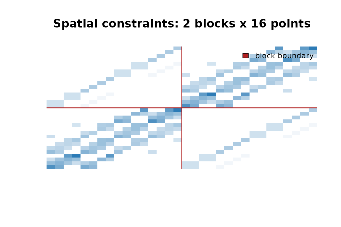

32x32 constraint matrix for two 4x4 spatial blocks. Diagonal blocks capture within-block spatial similarity; off-diagonal blocks link corresponding locations across blocks. The leading eigenvalue is 1 by construction.

The result is normalized so its largest eigenvalue equals 1 — it plugs directly into spectral methods that expect a properly scaled operator.

For heterogeneous blocks where each block has different feature observations, feature_weighted_spatial_constraints() extends this with per-block feature weighting.

Function reference

Function	What it builds
`spatial_adjacency()`	Symmetric spatial similarity from one coordinate set
`cross_spatial_adjacency()`	Rectangular similarity between two coordinate sets
`spatial_laplacian()`	Graph Laplacian L = D − A from coordinates
`spatial_smoother()`	Row-stochastic spatial averaging operator
`weighted_spatial_adjacency()`	Spatial adjacency blended with feature similarity
`bilateral_smoother()`	Edge-preserving spatial smoother
`spatial_constraints()`	Multi-block constraint matrix for repeated layouts
`feature_weighted_spatial_constraints()`	Multi-block constraints with per-block feature weighting
`normalize_adjacency()`	Row-normalize any adjacency matrix
`make_doubly_stochastic()`	Sinkhorn–Knopp doubly stochastic normalization

Where to go next

Feature-based graphs — graph_weights() and nnsearcher() build graphs from feature vectors rather than coordinates; see vignette("adjoin").
Diffusion — compute_diffusion_kernel() propagates information through any adjacency matrix, spatial or feature-based.
Label constraints — expand_label_similarity() combines spatial proximity with class labels for semi-supervised methods.
API reference — ?spatial_adjacency, ?spatial_constraints, ?bilateral_smoother for full parameter documentation.