Representational Similarity Analysis (RSA) in rMVPA

What problem does RSA solve?

You have a hypothesis about how stimuli relate to each other — by category, by visual similarity, by some embedding from a computational model. RSA tests whether the brain’s pattern of similarities across those stimuli matches your predicted pattern. The geometry of activity, not the activity itself, is the data.

The whole workflow is four steps: (i) build an MVPA dataset, (ii) supply one or more model RDMs (representational dissimilarity matrices), (iii) wrap them in an rsa_design(), (iv) fit with rsa_model() and run regionally or via searchlight.

A first win

Build a tiny dataset whose first half of trials shares one latent structure and the second half shares another, and a single model RDM that knows about it.

set.seed(2026)
ds <- gen_sample_dataset(D = c(8, 8, 8), nobs = 40, blocks = 4, nlevels = 2)

# A simple ordinal model RDM: nearby trial indices are predicted to be similar.
model_rdm <- as.matrix(stats::dist(seq_len(40)))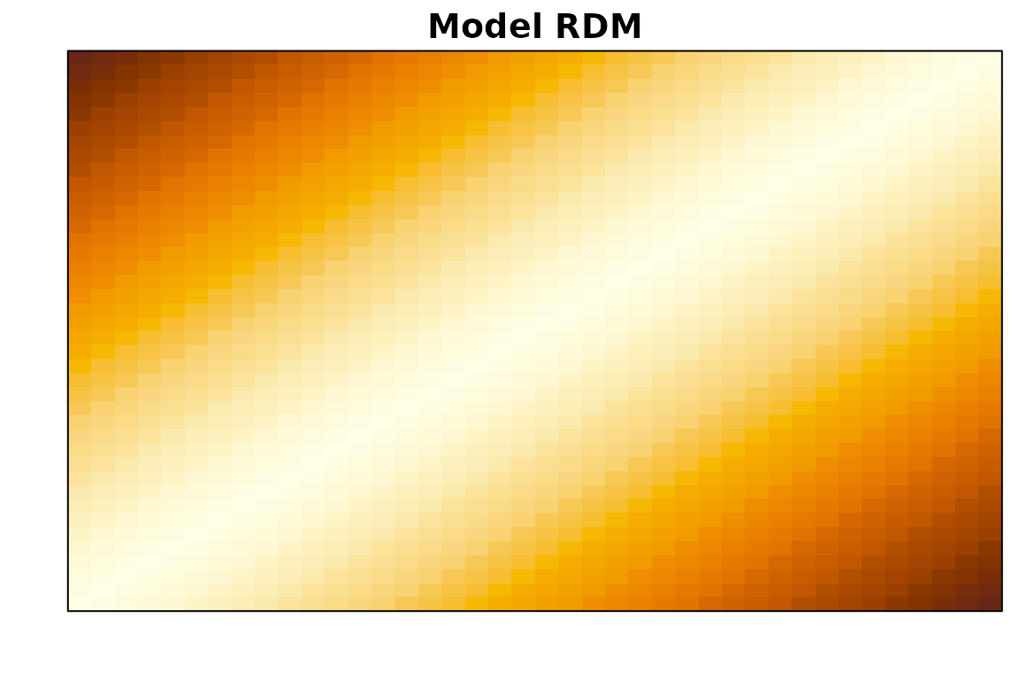

A model RDM. Dark cells = predicted small dissimilarity (similar items); bright cells = predicted large dissimilarity. Diagonal = 0.

Fit RSA in one regional pass:

des <- rsa_design(~ model_rdm, list(model_rdm = model_rdm),
                  block_var = ds$design$block_var)
mod <- rsa_model(ds$dataset, des, distmethod = "pearson", regtype = "pearson")
res <- run_regional(mod, region_mask = ds$dataset$mask, verbose = FALSE)
res$performance_table
#> # A tibble: 1 × 2
#>   roinum model_rdm
#>    <int>     <dbl>
#> 1      1  -0.00292

The performance_table row reports, per ROI, how well that ROI’s neural pair-dissimilarity vector tracks the model RDM. That’s the entire RSA core loop. The rest of this vignette covers the parts you’ll actually want to control: how to build model RDMs, how to combine multiple RDMs, how to handle correlated RDMs, and how to wire it into searchlight.

Basic concepts

Dissimilarity matrices

A dissimilarity matrix represents pairwise differences between conditions or stimuli. Each cell (i, j) quantifies how different two conditions are, and the matrix can be derived from either neural data or theoretical models. Common measures include correlation distance (1 − correlation) and Euclidean distance.

RSA workflow in rMVPA

In practice you (i) create an MVPA dataset, (ii) define one or more model dissimilarity matrices, (iii) build an RSA design, and (iv) fit and evaluate the RSA model.

Step-by-Step Example

1. Creating Sample Data

A larger synthetic dataset for the rest of the walkthrough:

dataset <- rMVPA::gen_sample_dataset(D = c(20, 20, 8), nobs = 80, blocks = 4)

2. Creating Model Dissimilarity Matrices

You can use different types of dissimilarity matrices:

# Method 1: Using dist() on feature vectors
model_features <- matrix(rnorm(80*10), 80, 10)  # 80 trials, 10 features
model_rdm <- dist(model_features)  # Default is Euclidean distance

# Method 2: Direct correlation distance matrix
model_matrix <- 1 - cor(t(model_features))  # Correlation distance

3. Creating an RSA Design

The RSA design specifies how to compare neural and model dissimilarity patterns:

# Basic design with one model RDM
basic_design <- rsa_design(
  formula = ~ model_rdm,
  data = list(model_rdm = model_rdm),
  block_var = factor(dataset$design$block_var)
)

# Design with multiple model RDMs
model_rdm2 <- dist(matrix(rnorm(80*10), 80, 10))
complex_design <- rsa_design(
  formula = ~ model_rdm + model_rdm2,
  data = list(
    model_rdm = model_rdm,
    model_rdm2 = model_rdm2
  ),
  block_var = factor(dataset$design$block_var),
  keep_intra_run = FALSE  # Exclude within-run comparisons
)

Decorrelating correlated model RDMs

Sometimes your model RDMs are not independent hypotheses. CNN layer RDMs are a common example: layers such as VGG-16 layer 4, 7, 11, and 16 are ordered and often share substantial representational structure. If you enter these RDMs directly into a multiple-RDM RSA model, shared geometry can make the individual layer effects hard to interpret.

rdm_decorrelate() is a preprocessing helper for this situation. It works on the lower-triangular RDM vectors, estimates layer-specific innovation RDMs, and returns adjusted RDMs that can be passed directly to rsa_design().

set.seed(12)

shared_visual <- matrix(rnorm(80 * 4), 80, 4)
layer_noise <- lapply(c(0.9, 0.7, 0.5, 0.35), function(sd) {
  matrix(rnorm(80 * 4, sd = sd), 80, 4)
})

cnn_features <- Map(function(noise, weight) {
  base::scale(weight * shared_visual + noise)
}, layer_noise, c(0.45, 0.60, 0.75, 0.90))
names(cnn_features) <- c("vgg4", "vgg7", "vgg11", "vgg16")

cnn_rdms <- lapply(cnn_features, dist)

raw_rdm_vectors <- vapply(cnn_rdms, as.vector, numeric(length(cnn_rdms[[1]])))
round(cor(raw_rdm_vectors, method = "spearman"), 2)
#>        vgg4  vgg7 vgg11 vgg16
#> vgg4   1.00 -0.01  0.08  0.09
#> vgg7  -0.01  1.00  0.32  0.30
#> vgg11  0.08  0.32  1.00  0.56
#> vgg16  0.09  0.30  0.56  1.00

The raw RDM correlations show how much representational geometry is shared across the model layers. The ordered innovation method treats the supplied order as meaningful: later-layer RDMs are decomposed into the part predicted by earlier layer innovations and the residual layer-specific component.

decorrelated <- rdm_decorrelate(
  cnn_rdms,
  method = "ordered_innovation",
  similarity = "spearman",
  epsilon = 0.05,
  gamma_grid = seq(0, 1, by = 0.05)
)

decorrelated$mean_abs_cor_before
#> [1] 0.2258285
decorrelated$mean_abs_cor_after
#> [1] 0.04841876
decorrelated$preservation
#>      vgg4      vgg7     vgg11     vgg16 
#> 1.0000000 1.0000000 0.9479340 0.9067018

The result records both the decorrelation achieved and how much each adjusted RDM still resembles the original. The adjusted RDMs are ordinary dist objects, so they can be used in a standard RSA design.

cnn_design <- rsa_design(
  formula = ~ vgg4 + vgg7 + vgg11 + vgg16,
  data = decorrelated$rdms,
  block_var = factor(dataset$design$block_var),
  keep_intra_run = FALSE
)

Use this when you want to test ordered, related model geometries while reducing shared RSA structure among them. The adjusted RDMs should be interpreted as layer-specific representational innovations, not as ordinary covariance shrinkage estimates.

4. Creating and Running an RSA Model

The rsa_model() function supports different methods for computing neural dissimilarities and analyzing relationships:

# Create MVPA dataset
dset <- mvpa_dataset(dataset$dataset$train_data, mask=dataset$dataset$mask)

# Create RSA model with different options
rsa_spearman <- rsa_model(
  dataset = dset,
  design = basic_design,
  distmethod = "spearman",  # Method for computing neural dissimilarities
  regtype = "spearman"      # Method for comparing neural and model RDMs
)

# Run searchlight analysis
results <- run_searchlight(
  rsa_spearman,
  radius = 4,
  method = "standard"
)

Advanced Features

Multiple Comparison Methods

rMVPA supports several methods for comparing neural and model RDMs:

# Pearson correlation
rsa_pearson <- rsa_model(dset, basic_design, 
                        distmethod = "pearson", 
                        regtype = "pearson")

# Linear regression
rsa_lm <- rsa_model(dset, basic_design, 
                    distmethod = "spearman", 
                    regtype = "lm")

# Rank-based regression
rsa_rfit <- rsa_model(dset, basic_design, 
                      distmethod = "spearman", 
                      regtype = "rfit")

Handling Run Structure

RSA can account for the run/block structure of fMRI data. A critical consideration in fMRI analysis is whether to include comparisons between patterns from the same run.

Understanding keep_intra_run

The keep_intra_run = FALSE parameter tells RSA to exclude comparisons between patterns within the same run/block. This is important because:

Temporal Autocorrelation: BOLD responses within the same run are temporally autocorrelated
Scanner Drift: Within-run patterns may share scanner drift effects
Physiological Noise: Within-run patterns may share structured noise from breathing, heart rate, etc.

Here’s a visualization of what keep_intra_run = FALSE does:

# Create a small example with 2 runs, 4 trials each
mini_data <- matrix(1:8, ncol=1)  # Trial numbers 1-8
run_labels <- c(1,1,1,1, 2,2,2,2)  # Two runs with 4 trials each

# Create distance matrix
d <- dist(mini_data)
d_mat <- as.matrix(d)

# Show which comparisons are kept (TRUE) or excluded (FALSE)
comparison_matrix <- outer(run_labels, run_labels, "!=")
# Only show lower triangle to match distance matrix structure
comparison_matrix[upper.tri(comparison_matrix)] <- NA

# Display the matrices
cat("Trial numbers:\n")
#> Trial numbers:
print(matrix(1:8, nrow=8, ncol=8)[lower.tri(matrix(1:8, 8, 8))])
#>  [1] 2 3 4 5 6 7 8 3 4 5 6 7 8 4 5 6 7 8 5 6 7 8 6 7 8 7 8 8
cat("\nRun comparisons (TRUE = across-run, FALSE = within-run):\n")
#> 
#> Run comparisons (TRUE = across-run, FALSE = within-run):
print(comparison_matrix[lower.tri(comparison_matrix)])
#>  [1] FALSE FALSE FALSE  TRUE  TRUE  TRUE  TRUE FALSE FALSE  TRUE  TRUE  TRUE
#> [13]  TRUE FALSE  TRUE  TRUE  TRUE  TRUE  TRUE  TRUE  TRUE  TRUE FALSE FALSE
#> [25] FALSE FALSE FALSE FALSE

When we create an RSA design with keep_intra_run = FALSE:

# Create design excluding within-run comparisons
blocked_design <- rsa_design(
  formula = ~ model_rdm,
  data = list(model_rdm = model_rdm),
  block_var = factor(dataset$design$block_var),
  keep_intra_run = FALSE  # Exclude within-run comparisons
)

This creates an RSA design that includes only between‑run comparisons, excludes within‑run pairs, and focuses the analysis on more reliable across‑run similarities.

When to use keep_intra_run = FALSE

Set keep_intra_run = FALSE when your design includes multiple runs and you want to control for temporal autocorrelation and run‑specific noise; this is the conservative choice for most confirmatory analyses. Keeping within‑run comparisons (keep_intra_run = TRUE, the default) can be reasonable in short‑run designs, when sample size is limited, or for exploratory work where maximizing comparisons is more important than strict control of temporal structure.

Visualizing Results

You can examine and visualize the RSA results:

# Extract the searchlight map
rsa_map <- results$results$model_rdm

# Compute range of correlation values
rsa_values <- neuroim2::values(rsa_map)
range(rsa_values, na.rm = TRUE)
#> [1] -0.06774093  0.06292384

# Basic summary of the searchlight result
print(results)
#> 
#>  Searchlight Analysis Results 
#> 
#> - Coverage 
#>   - Voxels/Vertices in Mask:  3,200 
#>   - Voxels/Vertices with Results:  3,200 
#> - Output Maps (Metrics) 
#>   -  model_rdm  (Type:  DenseNeuroVol )

# Save results (commented out)
# neuroim2::write_vol(rsa_map, "RSA_results.nii.gz")

Summary

The rMVPA package provides a comprehensive RSA implementation with flexible model specification, multiple dissimilarity computation methods, and support for complex experimental designs with run/block structures. It integrates seamlessly with searchlight analysis and offers various statistical approaches including correlation, regression, and rank-based methods.

When using RSA in rMVPA, carefully consider your experimental design when setting block variables and intra-run parameters, choose distance methods that match your theoretical framework, and select statistical approaches appropriate for your analysis goals.

From within-ROI scores to ROI-to-ROI connectivity

Once you have RSA scores per ROI, a natural follow-up is “where else does this geometry live?” rsa_model() accepts return_fingerprint = TRUE, which stores a small per-ROI projection of the neural pair vector onto your model RDM subspace. model_space_connectivity() then turns those fingerprints into ROI-by-ROI representational connectivity in one call. The same flag also feeds k-means anchor maps for searchlight runs without materialising an n_centers × n_centers matrix. See vignette("Model_Space_Connectivity") for the full workflow, including cross-domain pair designs (pair_rsa_design(..., pairs = "between")).

References

Kriegeskorte et al. (2008). Representational similarity analysis - connecting the branches of systems neuroscience. Front Syst Neurosci.
Nili et al. (2014). A toolbox for representational similarity analysis. PLoS Comput Biol.

Bradley Buchsbaum

2026-05-08