Partial Least Squares Correlation (PLSC) with Inference
PLSC.Rmd1. What this vignette covers
This walk-through shows how to:
- Fit a Behavior-style PLSC model (
plsc()). - Inspect latent variables (LVs) and scores.
- Run a permutation test to decide how many LVs are significant.
- Use bootstrap ratios to identify stable loadings, with simple visualizations.
The workflow is intentionally small so the vignette runs quickly; for applied analyses, increase the number of permutations and bootstraps.
2. Simulate coupled X/Y blocks
n  <- 80   # subjects
pX <- 8    # brain/features
pY <- 5    # behavior
d  <- 2    # true latent dimensions

# orthonormal loadings
Vx_true <- qr.Q(qr(matrix(rnorm(pX * d), pX, d)))
Vy_true <- qr.Q(qr(matrix(rnorm(pY * d), pY, d)))

F_scores <- matrix(rnorm(n * d), n, d)         # latent scores
noise    <- 0.10

X <- F_scores %*% t(Vx_true) + noise * matrix(rnorm(n * pX), n, pX)
Y <- F_scores %*% t(Vy_true) + noise * matrix(rnorm(n * pY), n, pY)
3. Fit PLSC
fit_plsc <- plsc(X, Y, ncomp = 3,                   # request a few extra comps
                 preproc_x = standardize(),         # correlation-scale
                 preproc_y = standardize())

fit_plsc$singvals
#> [1] 4.15551071 1.76186530 0.02831984
fit_plsc$explained_cov
#> [1] 8.475956e-01 1.523650e-01 3.936602e-05
4. Inspect scores (brain vs behavior)
scores_df <- data.frame(
  LV1_x = scores(fit_plsc, "X")[, 1],
  LV1_y = scores(fit_plsc, "Y")[, 1],
  LV2_x = scores(fit_plsc, "X")[, 2],
  LV2_y = scores(fit_plsc, "Y")[, 2]
)

ggplot(scores_df, aes(x = LV1_y, y = LV1_x)) +
  geom_point(alpha = 0.7) +
  geom_smooth(method = "lm", se = FALSE, color = "firebrick") +
  labs(x = "Behavior scores (LV1)", y = "Brain scores (LV1)",
       title = "Score association for LV1") +
  theme_minimal()
#> `geom_smooth()` using formula = 'y ~ x'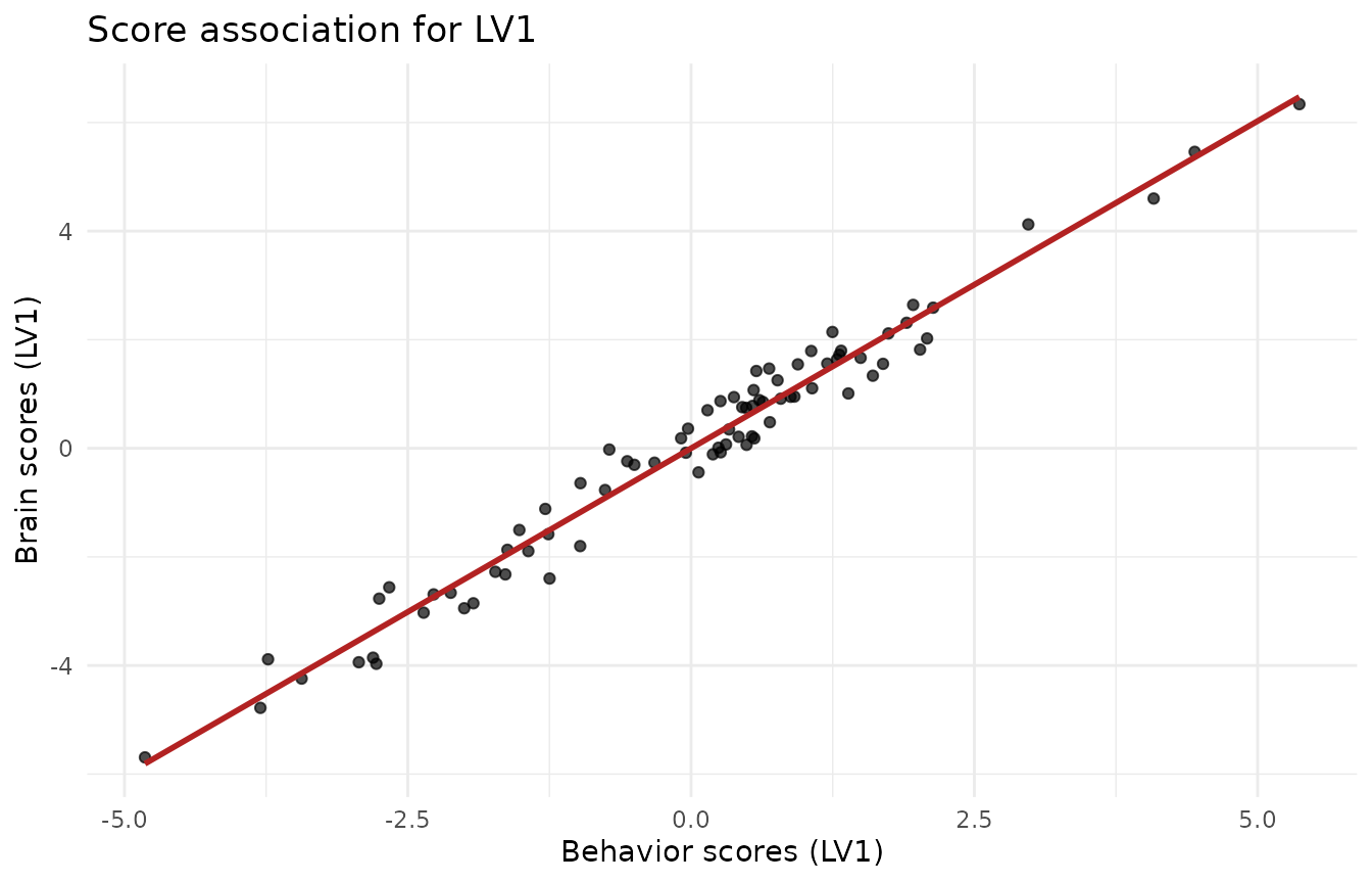
5. Permutation test: how many LVs?
Shuffle rows of Y to break the X–Y link and build an
empirical null for the singular values.
set.seed(123)
pt <- perm_test(fit_plsc, X, Y, nperm = 199, comps = 3, parallel = FALSE)
pt$component_results
#> # A tibble: 3 × 5
#>    comp observed  pval lower_ci upper_ci
#>   <int>    <dbl> <dbl>    <dbl>    <dbl>
#> 1     1   4.16   0.005   0.269    1.07
#> 2     2   1.76   0.005   0.0819   0.509
#> 3     3   0.0283 0.205   0.0140   0.0396
cat("Sequential n_significant (alpha = 0.05):", pt$n_significant, "\n")
#> Sequential n_significant (alpha = 0.05): 2
6. Bootstrap ratios for stable loadings
Bootstrap resamples subjects, re-fits PLSC, sign-aligns loadings, and
reports mean/SD (ratio ≈ Z).
Here we keep it light for the vignette; use ≥500–1000 in practice.
set.seed(321)
boot_plsc <- bootstrap(fit_plsc, nboot = 120, X = X, Y = Y, comps = 2, parallel = FALSE)

# X-loadings bootstrap ratios for LV1
df_bsr <- data.frame(
  variable = paste0("x", seq_len(pX)),
  bsr      = boot_plsc$z_vx[, 1]
)

ggplot(df_bsr, aes(x = reorder(variable, bsr), y = bsr)) +
  geom_hline(yintercept = c(-2, 2), linetype = "dashed", color = "grey50") +
  geom_col(fill = "#1f78b4") +
  coord_flip() +
  labs(x = NULL, y = "Bootstrap ratio (X loadings, LV1)",
       title = "Stable variables exceed |BSR| ≈ 2") +
  theme_minimal()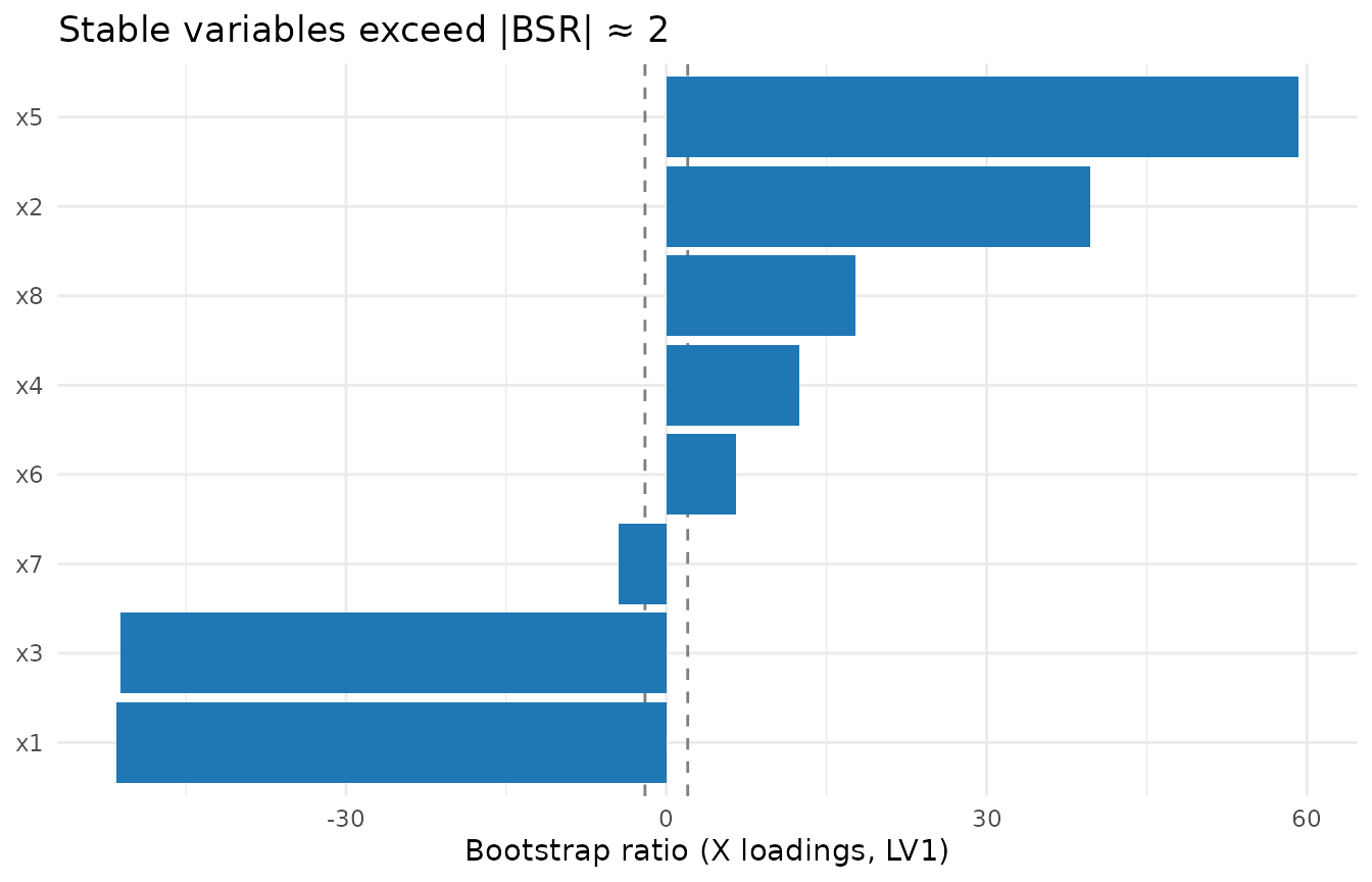
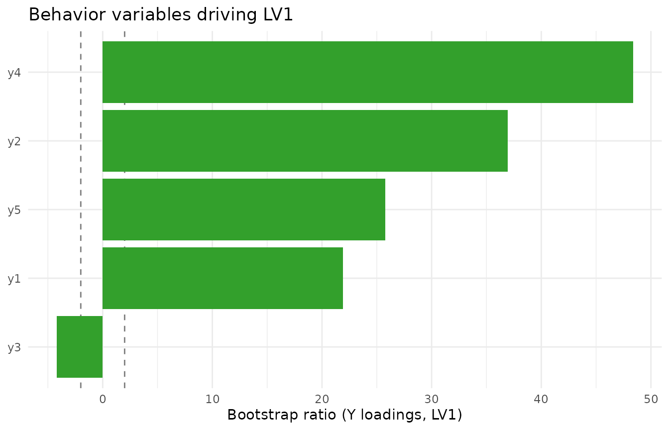
Do the same for Y loadings if needed:
7. Practical tips
- Use
standardize()to run PLSC on correlation scale (default here); switch tocenter()for covariance scale.
- Increase
nperm(e.g., 999) andnboot(≥500) for publication-grade inference.
- Interpret loadings only where bootstrap ratios exceed ~|2|, and only
for LVs that pass the permutation test.
- To visualise higher-dimensional loading maps (e.g., imaging),
replace the bar plots with your spatial plotting routine applied to
boot_plsc$z_vx.