Getting Started with fmriAR

Overview

fmriAR provides lightweight tools for estimating autoregressive (AR) or autoregressive–moving-average (ARMA) noise models from fMRI residuals and applying matched prewhitening to both design matrices and voxel-wise data. The C++ core keeps large-scale whitening fast, while the R interface stays compact and flexible.

This vignette walks through a typical workflow. We start by fitting an AR model to residuals from an initial OLS regression, then apply the resulting run-aware whitening plan to both the design matrix and the voxel data. With the innovations in hand we check that low-lag autocorrelation has been suppressed, explore how multiscale pooling stabilises parcel-level estimates, and finish with a brief look at ARMA models when MA structure remains.

Simulating data for the examples

To make the examples reproducible, we simulate a modest fMRI-style dataset with two runs, a small design matrix, and voxel-specific AR(2) noise.

library(fmriAR)
set.seed(42)

n_time <- 240
n_vox <- 60
runs <- rep(1:2, each = n_time / 2)

# Design matrix: intercept + task regressor
X <- cbind(
  intercept = 1,
  task = rep(c(rep(0, 30), rep(1, 30)), length.out = n_time)
)

# Generate voxel time-series with AR(2) noise
phi_true <- matrix(0, nrow = n_vox, ncol = 2)
phi_true[, 1] <- 0.5 + rnorm(n_vox, sd = 0.05)
phi_true[, 2] <- -0.2 + rnorm(n_vox, sd = 0.05)

Y <- matrix(0, n_time, n_vox)
innov <- matrix(rnorm(n_time * n_vox, sd = 1), n_time, n_vox)
for (v in seq_len(n_vox)) {
  for (t in seq_len(n_time)) {
    ar_part <- 0
    if (t > 1) ar_part <- ar_part + phi_true[v, 1] * Y[t - 1, v]
    if (t > 2) ar_part <- ar_part + phi_true[v, 2] * Y[t - 2, v]
    Y[t, v] <- ar_part + innov[t, v]
  }
}

# Add task signal to half the voxels
beta <- c(0, 1.5)
Y_signal <- drop(X %*% beta)
Y[, 1:30] <- sweep(Y[, 1:30], 1, Y_signal, "+")

# Residuals from initial OLS fit
coeff_ols <- qr.solve(X, Y)
resid <- Y - X %*% coeff_ols

Fitting an AR model

The primary entry point is fit_noise(). When method = "ar" and p = "auto", the function selects the AR order per run using BIC, then enforces stationarity.

plan_ar <- fit_noise(
  resid,
  runs = runs,
  method = "ar",
  p = "auto",
  p_max = 6,
  exact_first = "ar1",
  pooling = "run"
)

plan_ar
# fmriAR whitening plan
#   Method: AR
#   Orders: p = 2, q = 0
#   Pooling: run
#   Runs: 2 (1, 2)
#   Exact first-sample scaling: AR(1)
#   Coefficients:
#     1: phi = 0.485, -0.193
#     2: phi = 0.482, -0.196

The returned fmriAR_plan holds run-specific AR coefficients and metadata about the estimation procedure.

Whitening design and data matrices

whiten_apply() takes the plan, design matrix, and observed data and returns whitened versions that can be used in GLS estimation or downstream analyses.

whitened <- whiten_apply(plan_ar, X, Y, runs = runs)
str(whitened)
# List of 2
#  $ X: num [1:240, 1:2] 1 0.515 0.708 0.708 0.708 ...
#   ..- attr(*, "dimnames")=List of 2
#   .. ..$ : NULL
#   .. ..$ : chr [1:2] "intercept" "task"
#  $ Y: num [1:240, 1:60] -1.4936 -1.5949 -0.0306 -1.0101 -0.0617 ...

By default the function returns whitened X and Y. You can compute GLS coefficients with a single linear solve:

Xw <- whitened$X
Yw <- whitened$Y
beta_gls <- qr.solve(Xw, Yw[, 1:5])
beta_gls
#                 [,1]       [,2]        [,3]       [,4]       [,5]
# intercept -0.1785576 0.03768029 -0.04137929 0.08983252 0.03839622
# task       1.6659992 1.38144408  1.18152789 1.45707478 1.53914426

Inspecting innovations

The whitened residuals (innovations) should look close to white noise. The helper below computes the average absolute autocorrelation across voxels.

innov_var <- Yw - Xw %*% qr.solve(Xw, Yw)
lag_stats <- apply(innov_var, 2, function(y) {
  ac <- acf(y, plot = FALSE, lag.max = 5)$acf[-1]
  mean(abs(ac))
})
mean(lag_stats)
# [1] 0.05721336

For comparison, the same calculation on the pre-whitened residuals is typically much larger.

In this simulation the mean absolute autocorrelation over lags 1–5 drops by several fold after whitening; exact values vary with the random seed, but the whitened summary should be markedly smaller than the raw baseline.

lag_stats_raw <- apply(resid, 2, function(y) {
  ac <- acf(y, plot = FALSE, lag.max = 5)$acf[-1]
  mean(abs(ac))
})
mean(lag_stats_raw)
# [1] 0.140151

avg_acf <- function(mat, lag.max = 20) {
  acf_vals <- sapply(seq_len(ncol(mat)), function(j) {
    stats::acf(mat[, j], plot = FALSE, lag.max = lag.max)$acf
  })
  rowMeans(acf_vals)
}

lag_max <- 20
lags <- seq_len(lag_max)
acf_raw <- avg_acf(resid, lag.max = lag_max)
acf_white <- avg_acf(innov_var, lag.max = lag_max)

ylim <- range(c(acf_raw[-1L], acf_white[-1L], 0))
plot(lags, acf_raw[-1L], type = "h", lwd = 2, col = "#1b9e77",
     ylim = ylim, xlab = "Lag", ylab = "Average autocorrelation",
     main = "Mean autocorrelation across voxels")
lines(lags, acf_white[-1L], type = "h", lwd = 2, col = "#d95f02")
abline(h = 0, col = "grey70", lty = 2)
legend("topright",
       legend = c("Raw residuals", "Whitened innovations"),
       col = c("#1b9e77", "#d95f02"),
       lwd = 2, bty = "n")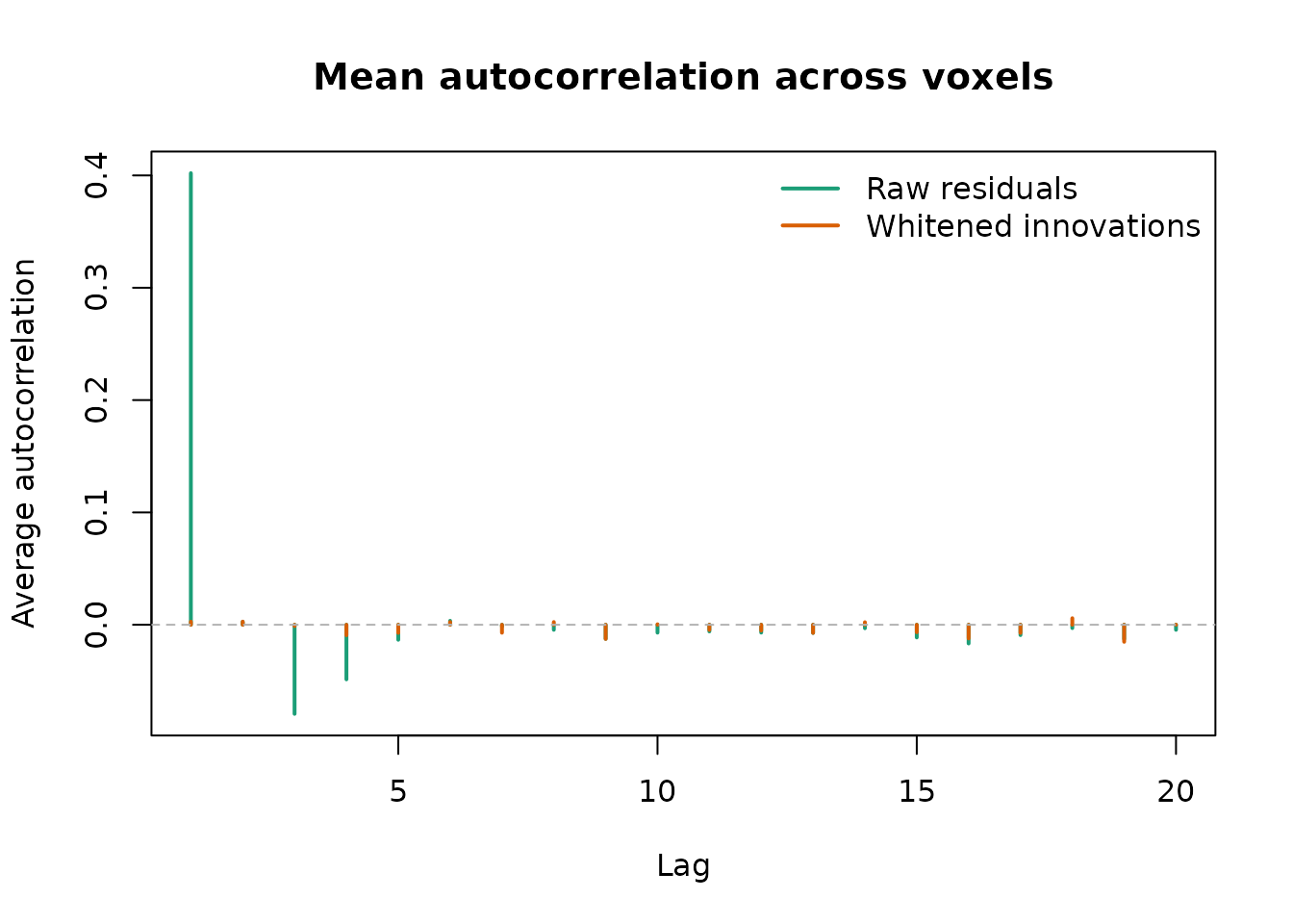

Average autocorrelation across voxels before and after whitening

Parcel pooling and multiscale shrinkage

When per-voxel residuals are noisy, you can pool information across parcels. The example below constructs synthetic parcels and uses the multiscale PACF-weighted shrinkage.

Under the hood, fit_noise(..., pooling = "parcel") builds parcel-level mean residual series at one or more spatial resolutions (fine/medium/coarse). Each parcel’s AR model is estimated with run-aware autocovariances, and then the coefficients are shrunk toward their parents by combining either partial autocorrelations (“pacf_weighted”) or autocovariance functions (“acvf_pooled”). The weights depend on parcel size, dispersion across voxels, and the number of runs, so larger or more homogeneous parcels lend more stability to their descendants while preserving stationarity for the final per-parcel filters.

parcels_fine <- rep(1:12, each = n_vox / 12)
parcels_medium <- rep(1:6, each = n_vox / 6)
parcels_coarse <- rep(1:3, each = n_vox / 3)

plan_parcel <- fit_noise(
  resid,
  runs = runs,
  method = "ar",
  p = "auto",
  p_max = 6,
  pooling = "parcel",
  parcels = parcels_fine,
  parcel_sets = list(
    fine = parcels_fine,
    medium = parcels_medium,
    coarse = parcels_coarse
  ),
  multiscale = "pacf_weighted"
)

plan_parcel$order
# p q 
# 6 0

When parcel pooling is requested, whiten_apply() returns X_by, a list of whitened design matrices per parcel, along with the voxel-wise Y innovations.

whitened_parcel <- whiten_apply(plan_parcel, X, Y, runs = runs, parcels = parcels_fine)
length(whitened_parcel$X_by)
# [1] 12

Fitting ARMA models

Some datasets require ARMA models to capture remaining MA structure. The workflow mirrors the AR case but sets method = "arma" and supplies orders (p, q).

plan_arma <- fit_noise(
  resid,
  runs = runs,
  method = "arma",
  p = 2,
  q = 1,
  hr_iter = 1
)

plan_arma$order
# p q 
# 2 1

ARMA whitening uses the same whiten_apply() interface.

whitened_arma <- whiten_apply(plan_arma, X, Y, runs = runs)
whitened_arma$X[1:5, ]
#      intercept task
# [1,] 1.0000000    0
# [2,] 0.4657323    0
# [3,] 0.5693939    0
# [4,] 0.6397975    0
# [5,] 0.6876133    0

AFNI-style restricted AR filters

If you need to replicate AFNI’s “restricted ARMA” family—real + complex AR roots with optional additive white noise—fmriAR exposes a stable wrapper via its compatibility interface: use compat$afni_restricted_plan() to construct matching whitening plans. This returns the same fmriAR_plan objects used elsewhere while keeping the main public API minimal.

The helper expects the AFNI root parameterisation (a real root a, complex pairs defined by radius/angle, and an optional MA(1) refinement) and can operate globally or per parcel. Because the interface mirrors AFNI’s internals, it is a convenient bridge when comparing pipelines or validating fmriAR against established AFNI analyses.

# Example: AFNI-style AR(3) with optional MA(1) term
roots <- list(a = 0.6, r1 = 0.7, t1 = pi / 6)

plan_afni <- compat$afni_restricted_plan(
  resid = resid,
  runs = runs,
  parcels = NULL,
  p = 3L,
  roots = roots,
  estimate_ma1 = TRUE
)

plan_afni$order

# Apply whitening just like any other plan
whitened_afni <- whiten_apply(plan_afni, X, Y, runs = runs)

Tip: set estimate_ma1 = FALSE to obtain the pure AR filter implied by the AFNI roots, or provide a list of root specifications keyed by parcel ID to drive parcel-specific filters that mirror AFNI’s voxel grouping.

Diagnostics and sandwich estimates

The package includes helpers for quick diagnostics and variance estimation:

# Autocorrelation diagnostics for whitened residuals
acorr <- acorr_diagnostics(Yw[, 1:3])
acorr
# $lags
#  [1]  1  2  3  4  5  6  7  8  9 10 11 12 13 14 15 16 17 18 19 20
# 
# $acf
#  [1]  0.392581599  0.360973704  0.310315389  0.322265370  0.374991747
#  [6]  0.210502166  0.223249048  0.235552972  0.217492041  0.143651583
# [11]  0.100407607  0.025318410  0.070841147  0.056705121  0.030469542
# [16]  0.010908172  0.003657289 -0.015876436 -0.048598733 -0.084495619
# 
# $ci
# [1] 0.1265175

# Sandwich standard errors from whitened residuals
sandwich <- sandwich_from_whitened_resid(whitened$X, whitened$Y[, 1:3])
sandwich$se
#           [,1]      [,2]      [,3]
# [1,] 0.1161948 0.1309954 0.1219902
# [2,] 0.1629742 0.1837334 0.1711027

Next steps

Explore the test suite in tests/testthat for additional usage patterns, including multiscale pooling and ARMA recovery checks.
Inspect the exported fmriAR_plan object with plan_info() to see per-run or per-parcel coefficients.
Combine whiten_apply() with GLS modelling packages to build end-to-end prewhitened analyses.

For production usage, consider benchmarking with your acquisition parameters and reviewing the package README for tuning options such as thread control and censor handling.

fmriAR Team

2025-10-18