Getting started with backend-aware matrices in amatrix

library(amatrix)

amatrix is for matrix-heavy code that already fits the Matrix idiom but needs a cleaner path to accelerated execution. You keep ordinary matrix inputs, wrap them once, and then use Matrix-compatible objects that carry backend preferences into linear algebra and model fitting.

This vignette uses one common workload: one design matrix, many response columns. By the end, you will have a backend-aware design matrix, a shared-design QR fit from many_lm(), and a compact way to inspect where amatrix plans to run each operation.

What do your inputs look like?

c(
  observations = nrow(X),
  predictors = ncol(X),
  responses = ncol(Y)
)
#> observations   predictors    responses 
#>          120            6            8

The design matrix X is an ordinary dense R matrix with one row per observation and one column per predictor. The response matrix Y has the same number of rows, but each column is a separate regression target that shares the same design.

What is the quickest end-to-end path?

X_am <- adgeMatrix(X)
fit <- many_lm(X_am, Y, method = "qr", include_fitted = TRUE, include_residuals = TRUE)
dim(coef(fit))
#> [1] 6 8

adgeMatrix() is the main dense-matrix constructor. many_lm() then fits all response columns against the same design in one call and returns a coefficient matrix with one column per response.

How does amatrix decide where to run?

amatrix_backend_status()[, c("name", "available", "precision_modes", "residency_capable")]
#>        name available precision_modes residency_capable
#> 1 arrayfire     FALSE            <NA>             FALSE
#> 2       cpu      TRUE     strict,fast             FALSE
#> 3     metal     FALSE            <NA>             FALSE
#> 4       mlx     FALSE            <NA>             FALSE
#> 5    opencl     FALSE            <NA>             FALSE

The status table tells you which backends are registered on the current machine and whether they are usable right now. A backend can be registered but unavailable, in which case the same code still has a predictable CPU fallback.

plan <- amatrix_backend_plan(X_am, "qr")
plan[c("chosen", "chosen_path", "requested_precision")]
#> $chosen
#> [1] "cpu"
#> 
#> $chosen_path
#> [1] "cold"
#> 
#> $requested_precision
#> [1] "strict"

This plan is the compact view of a dispatch decision. You can see which backend was chosen, whether the operation will run as a cold or resident path, and which precision contract the object is requesting.

When does shared-design caching help?

The main reason to use amatrix for repeated regression is that the design-matrix factorization can be reused across calls when X stays the same. That matters when you fit many batches of responses against one shared design.

X_cache_am <- adgeMatrix(X)
fit_a <- many_lm(X_cache_am, Y[, 1:4, drop = FALSE], method = "qr", cache = TRUE)
fit_b <- many_lm(X_cache_am, Y[, 5:8, drop = FALSE], method = "qr", cache = TRUE)

c(first_call = fit_a$cache_reused, second_call = fit_b$cache_reused)
#>  first_call second_call 
#>       FALSE        TRUE

With a fresh backend-aware copy of X, the first call computes and stores the QR factorization for that design. The second call reuses it because the design matrix is unchanged.

What should you inspect after a fit?

summary_tbl <- data.frame(
  response = colnames(Y),
  rss = round(fit$rss, 3),
  sigma2 = round(fit$sigma2, 4),
  r2 = round(r2, 3)
)

knitr::kable(summary_tbl, align = "lrrr")

	response	rss	sigma2	r2
response_1	response_1	4.402	0.0386	0.980
response_2	response_2	6.406	0.0562	0.964
response_3	response_3	3.696	0.0324	0.961
response_4	response_4	4.614	0.0405	0.992
response_5	response_5	4.157	0.0365	0.990
response_6	response_6	3.890	0.0341	0.994
response_7	response_7	4.913	0.0431	0.956
response_8	response_8	4.789	0.0420	0.949

rss and sigma2 tell you how much unexplained variation remains in each response. Here the fitted models recover most of the signal because the responses were generated from a shared linear design with modest noise.

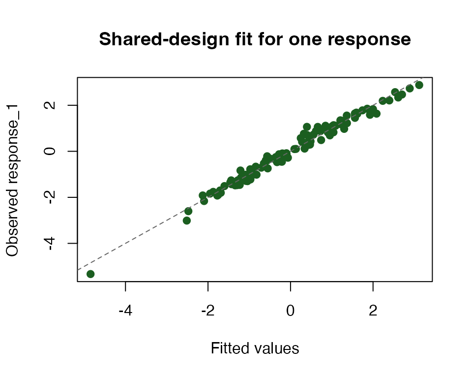
The points fall close to the identity line, which matches the high r2 values from the hidden checks and the small residual variances in the summary table.

How do you ask for a fast backend?

The CPU path above is the safest default because it runs everywhere. On a machine with an available accelerator backend, the code shape stays the same and you only change the constructor metadata:

X_fast <- adgeMatrix(X, mode = "fast")
fit_fast <- many_lm(X_fast, Y, method = "qr", cache = TRUE)

coef(fit_fast)

If you are writing library code, the default path is still to wrap once at the boundary and keep the rest of the code generic:

X_am <- as_adgeMatrix(X, mode = "fast")
fit <- many_lm(X_am, Y, method = "qr", cache = TRUE)

That per-object path does not require session-global setters or a hardcoded backend name. amatrix will prefer an available fast-capable accelerator automatically and fall back to CPU when none is available.

If a caller wants to flip defaults for one local block instead of one object, use with_amatrix():

with_amatrix(policy = "auto", precision = "fast", {
  X_am <- as_adgeMatrix(X)
  fit <- many_lm(X_am, Y, method = "qr", cache = TRUE)
})

Use amatrix_bind_resident() only when you need to optimize a particularly hot repeated path.

Where next?

The next functions to explore are adgeMatrix(), many_lm(), amatrix_backend_status(), and amatrix_explain(). If you want to audit a single operation more deeply, start with amatrix_backend_plan() and then compare that compact plan to the printed explanation from amatrix_explain().