Fit a Blocked Voxelwise Banded-Ridge Encoding Model

You have several time-aligned feature spaces—for example, visual motion, audio, and semantic features—and one BOLD response at every voxel. You want to predict each voxel on observations the model never saw, while allowing different feature spaces and different voxels to need different amounts of regularization. Randomly splitting a time series would leak temporal context, so the validation units must remain intact.

This guide builds that analysis with three contiguous stimulus segments. By the end, you will have voxelwise outer out-of-fold predictions, MSE, correlation, R2, the alpha and feature-space weights selected inside each outer training set, and optional predictive leave-one-band-out delta R2 maps.

What are the inputs?

Rows of the predictor matrix must align exactly with volumes in the image series. blocks() receives numbers of columns, not column indices. The design owns both feature-band membership and the training block metadata, so the model cannot receive a second, conflicting band specification.

features <- feature_sets(
  example$X,
  blocks(visual = 4, semantic = 4)
)

design <- feature_sets_design(
  features,
  block_var_train = example$blocks,
  time_series = TRUE
)

The example has 36 observations, eight predictors in two named bands, three independent temporal segments, and 18 active voxels.

Aligned inputs for the worked example.

observations	predictors	feature_bands	temporal_blocks	active_voxels
36	8	2	3	18

How do you fit the model safely?

The outer folds estimate generalization. The inner folds choose hyperparameters using only the corresponding outer-training rows. Because the design declares a time series, rMVPA refuses an unsafe random split unless you provide intact blocks or an explicit temporal purge.

model <- banded_ridge_model(
  example$dataset, design,
  outer_crossval = 3, tune_crossval = 2,
  theta_method = "grid", theta_grid_points = 3,
  target_batch_size = 7, return_predictions = TRUE,
  delta_sets = "all"
)

result <- run_banded_ridge(model)

alphas is left at its default, "auto", which places nine penalties across six decades around the scale at which the penalty starts to change this design’s fit. That scale is a property of the design, not a constant: the solver standardizes every training column and scales band b by sqrt(theta_b), so alpha competes with cross-product eigenvalues that average (n - 1) * mean(D_b) / min(n - 1, p). It grows with the number of rows and with band width, which is why a design with a few thousand timepoints needs penalties orders of magnitude larger than one with a few dozen.

signif(model$alpha_grid, 3)
#> [1] 1.75e-02 9.84e-02 5.53e-01 3.11e+00 1.75e+01 9.84e+01 5.53e+02 3.11e+03
#> [9] 1.75e+04

outer_crossval also accepts a cross_validation object, so blocked_cross_validation(example$blocks) selects the same block-wise outer folds used elsewhere in rMVPA. Integer counts and cross_validation objects have purge applied to their training rows, whereas a hand-built fold list is validated as supplied. tune_crossval can be omitted: the default uses at most five inner folds, limited by the blocks (or rows, when none are declared) available inside each outer-training set, and inner tuning is skipped entirely when only one candidate survives the alpha/theta scopes.

The compact result table is already in original voxel order. These are pooled outer out-of-fold metrics: every observation contributes once, from the outer fold in which it was held out.

head(result$metrics)
#>   voxel_index response n_obs       mse correlation        r2
#> 1           1  voxel_1    36 0.4212985   0.9188365 0.8425157
#> 2           2  voxel_2    36 0.3902411   0.9558373 0.9133813
#> 3           3  voxel_3    36 0.3619358   0.9620976 0.9256266
#> 4           4  voxel_4    36 0.5749462   0.7747922 0.5937547
#> 5           5  voxel_5    36 0.5011491   0.5359127 0.2762339
#> 6           6  voxel_6    36 0.3534999   0.9166569 0.8398795

The hyperparameter table is deliberately fold-specific. A single averaged alpha or theta map is convenient for visualization, but this table is the exact record of what generated each fold’s predictions.

head(result$hyperparameters[, c(
  "voxel_index", "outer_fold", "alpha",
  "theta_visual", "theta_semantic", "inner_score"
)])
#>   voxel_index outer_fold      alpha theta_visual theta_semantic inner_score
#> 1           1     fold_1 0.09840973          0.5            0.5   0.5676847
#> 2           1     fold_2 0.09840973          1.0            0.0   0.2934400
#> 3           1     fold_3 0.55339859          1.0            0.0   0.5994161
#> 4           2     fold_1 0.09840973          1.0            0.0   0.5679984
#> 5           2     fold_2 0.01750000          1.0            0.0   0.5735952
#> 6           2     fold_3 0.55339859          1.0            0.0   0.3304154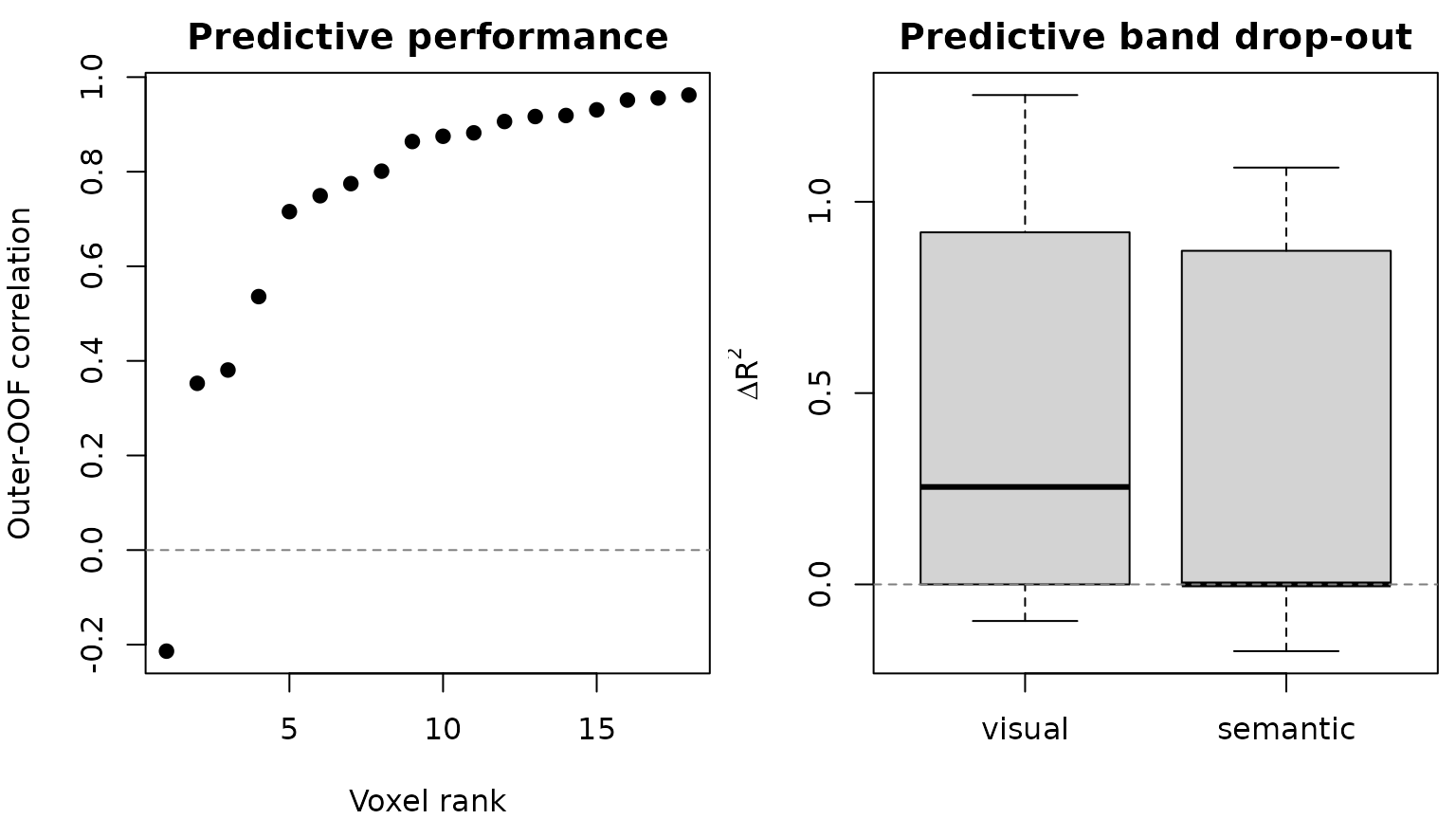

Positive and negative values are both meaningful. A negative delta means the independently retuned reduced model predicted better in these finite samples; the value is never clipped.

Did the tuning grid contain the optimum?

A tuning grid that stops short of the optimum does not fail. Every response simply takes the largest penalty on offer, the refit is under-penalized, and the maps and delta R2 values come back fully populated and wrong. Read result$selection_diagnostics before anything else.

result$selection_diagnostics$alpha[, c(
  "model", "modal_alpha", "share_at_grid_min", "share_at_grid_max",
  "share_interior", "saturated"
)]
#>              model  modal_alpha share_at_grid_min share_at_grid_max
#> 1             full 5.533986e-01        0.14814815         0.0000000
#> 2   without_visual 1.750000e+04        0.09259259         0.3148148
#> 3 without_semantic 3.111989e+00        0.09259259         0.2222222
#>   share_interior saturated
#> 1      0.8518519     FALSE
#> 2      0.5925926     FALSE
#> 3      0.6851852     FALSE

The signature of a usable grid is an interior modal selection: most responses chose an alpha that is neither the smallest nor the largest available, so the grid brackets the optimum rather than truncating it. saturated is set when 95% of a model’s selections take one end of the grid, or when the two ends hold 95% between them, and run_banded_ridge() warns. Both forms matter. Alpha is tuned per response by default, so a mask that mixes predictable voxels with unpredictable ones sends its boundary mass to opposite ends — the noise voxels want more penalty than the ceiling offers, the signal voxels less than the floor — and neither end alone need look alarming while almost nothing lands inside. Widen alphas until the modal selection moves inside.

$fit answers the second question, which is independent of the grid: did the model predict at all?

result$selection_diagnostics$fit
#>              model n_responses n_scored  median_r2   mean_r2 share_r2_positive
#> 1             full          18       18  0.7527416 0.6054574         0.9444444
#> 2   without_visual          18       18 -0.0218104 0.1722848         0.3333333
#> 3 without_semantic          18       18  0.2720315 0.3170440         0.6666667

A median outer out-of-fold R2 below -0.05 means the fit predicts worse than the mean of the data it was scored on, and run_banded_ridge() warns about that separately. Nothing downstream of such a fit describes explained variance — in particular, the leave-one-band-out deltas are then differences between two models that both fail.

Which loss and which score are you reading?

Three quantities answer different questions:

1. inner_score is the selection loss. The default is MSE computed from inner out-of-fold predictions within one outer-training set. Correlation and R2 are explicit opt-in selection criteria.
2. mse, correlation, and r2 in result$metrics are descriptive scores computed after concatenating the outer out-of-fold predictions. They are not the inner selection scores.
3. delta_cv_r2_<band> is R2_full - R2_without_band, using the same outer test rows for both models. Each reduced model is tuned again. This is a predictive leave-one-band-out effect, not an additive unique/shared variance decomposition, so effects need not sum to the full-model R2.

The fitted objective for a fixed candidate is

$$\widehat B = \arg\min_B \lVert Y - XB \rVert_F^2 + \sum_g \frac{\alpha}{\theta_g}\lVert B_g \rVert_F^2,$$

where non-negative theta values sum to one. theta_g = 0 excludes a band exactly. The squared-error term is not divided by the number of observations, so alpha is on the scale of the training cross-product. Centering and scaling are learned separately inside every training split. Equal theta values recover ordinary ridge after accounting for scale: with G bands and ordinary ridge penalty lambda, use theta_g = 1/G and alpha = lambda/G.

What is retained, and what can become large?

The constructor resolves the solver and estimates retained output storage before fitting. The default keeps metrics and hyperparameters but not the full prediction matrix, coefficients, or nested diagnostics. Request those outputs only when you need them.

Decision and retained-storage estimate available before fitting.

chosen_solver	reason	predictions_MiB	attribution_MiB	total_retained_MiB
direct	measured small-p direct threshold p <= 64 and storage fits	0.0148	0.0074	0.0222

Use weight_retention = "primal" for outer-fold coefficient matrices or "dual" for outer-fold sample-space weights. max_retained_mb refuses an unsafe request before allocation; weight_overflow = "none" may explicitly fall back to no weights. memory_limit_mb independently guards solver intermediates and caps the retained decomposition cache: band Gram matrices are cached once per training split and shared across theta candidates and drop-out models, and least-recently-used entries are evicted (and recomputed on demand) once the cap is reached, so the limit changes reuse but never results. Runtime provenance records the chosen solver, chunk manifest, decomposition, band-Gram reuse, and eviction counts, maximum chunk result size, and the B+1 cost of requested drop-out models.

For F outer folds, K inner folds, T theta candidates, A alphas, and response chunks of size B, tuning evaluates approximately F * K * T * A candidate fits per conceptual model and then performs outer refits. Optimized paths reuse a decomposition across alpha values only when the training rows and theta are unchanged. Changing theta changes the scaled design/kernel and requires another decomposition; there is no claim of one decomposition for the entire search.

What did the issue #70 simulation show when rerun?

Issue #70 reported a large relative gain from per-voxel penalties in one simulation. The reproducibility script installed at benchmarks/banded_ridge_issue70.R defines a concrete successor: two bands, 40 voxels at SNR 1.0/0.4/0.0, six contiguous outer segments, nested tuning, and 30 declared seeds. It compares shared alpha/theta with response-specific alpha/theta and reports the absolute OOF-correlation change.

Issue #70 successor simulation. Intervals are empirical 2.5% and 97.5% quantiles of replication-level mean absolute gains.

	SNR	shared_r	response_specific_r	absolute_gain	gain_q025	gain_q975
0	0.0	-0.014	-0.023	-0.010	-0.080	0.047
0.4	0.4	0.269	0.222	-0.048	-0.069	-0.030
1	1.0	0.599	0.589	-0.010	-0.025	0.015

This registered variant did not reproduce the earlier 78% claim. At SNR 0.4, response-specific tuning changed OOF correlation by about -0.048 in absolute units (replication interval about -0.069 to -0.030). The result is specific to this data-generating process, MSE selection rule, and candidate grid; it is neither evidence that shared tuning is universally better nor a correctness test. Across pure-noise voxels, the replication-level mean response-specific correlation was close to zero (about -0.023; empirical 95% interval about -0.092 to 0.013). The direct/SVD/dual oracles, leakage mutations, and attribution adversaries provide correctness evidence instead.

How does this relate to other ridge tools?

Choose by estimand and execution environment, then compare on identical folds, preprocessing, candidate sets, and response scoring.

Tool	Useful when	Important comparison boundary
Ordinary ridge	One common penalty across all feature columns is the scientific model	In rMVPA, use fixed equal theta and convert ordinary lambda to alpha = lambda/G
glmnet	You need elastic-net/lasso paths or its established sparse-matrix tooling	mgaussian is a multi-task group penalty across responses; its objective scaling and standardization conventions differ
multiridge	You want its multi-penalty CV or marginal-likelihood workflows for high-dimensional data blocks	Its optimization, preprocessing, and response model are not assumed to be numerically identical to this nested voxelwise estimand
himalaya	You want Python, CPU/GPU backends, or multiple-kernel/group-ridge solvers at very large target counts	It is an external parity target, not an rMVPA dependency; align folds, centering, alpha/theta parameterization, and precision before comparing

The bundled fixed-shape performance receipt likewise characterizes, rather than proves superiority. On the recorded Apple M3 Max / R 4.5.1 run, the n = 60, p = 512, V = 12 public workflow took median 0.226 seconds with the direct backend and 0.099 seconds with each optimized backend over five runs. The solver planner estimated 2.15 MB, 0.33 MB, and 0.17 MB of intermediate storage respectively. Wall times are tracked as snapshots; CI enforces structural shape, batching, allocation, cache, and numerical-parity contracts instead of brittle timing cutoffs.

Where should you go next?

Use ?banded_ridge_model for the complete objective, candidate, storage, and failure contracts; ?run_banded_ridge for the result schema and regional batching rules; and vignette("CrossValidation") for broader validation design. For temporally ordered data, decide the independent blocks or purge from the acquisition and stimulus design before choosing a solver.