Feature-RSA Connectivity: ROI-to-ROI Generalization and Offset Control

Feature-RSA normally stops at one ROI at a time: does the learned geometry explain held-out data in that ROI? Sometimes the next question is larger. If ROI 3 learns a useful geometry, does that geometry show up in ROI 7 as well? If one target ROI is easy for every source ROI, how do you separate that global effect from pair-specific transfer?

feature_rsa_connectivity() and feature_rsa_cross_connectivity() answer those questions at the level of representational geometry rather than voxel weights. That matters because ROI sizes can differ and you still get a clean ROI x ROI summary.

What does the cross-ROI matrix look like?

The quick example below fits feature-RSA in four synthetic parcels, stores the predicted and observed RDM vectors for each ROI, and then builds the asymmetric ROI_i -> ROI_j matrix.

conn_example <- build_connectivity_example()

knitr::kable(round(conn_example$cross_raw, 2))

1	2	3	4
0	0.03	-0.02	-0.05
0	0.07	-0.03	-0.02
0	0.02	0.02	-0.05
0	0.03	-0.01	-0.01

Asymmetric ROI x ROI cross-connectivity. Rows are source ROIs (the geometry learned there), columns are target ROIs (the geometry observed there). Diagonal = within-ROI feature-RSA fit; off-diagonals = cross-ROI generalization.

Rows are source ROIs: the predicted geometry learned in that ROI. Columns are target ROIs: the observed geometry in held-out data from that ROI. The diagonal is the familiar within-ROI feature-RSA fit. The off-diagonal entries are cross-ROI generalization scores.

How do you extract the per-ROI geometry?

The only extra requirement is return_rdm_vectors = TRUE when you fit feature_rsa_model(). That stores compact lower-triangle RDM vectors for each ROI, and feature_rsa_rdm_vectors() pulls them into a tibble.

head(conn_example$vecs[, c("roinum", "n_obs")])
#> # A tibble: 4 × 2
#>   roinum n_obs
#>    <int> <int>
#> 1      1    36
#> 2      2    36
#> 3      3    36
#> 4      4    36

This is the bridge between ordinary per-ROI feature-RSA and the ROI-to-ROI summaries. You still fit ROI models in the usual way. The difference is that you keep the predicted and observed geometry vectors around for a second-stage comparison.

When do you want the symmetric matrix?

feature_rsa_connectivity() asks whether the predicted geometries themselves are similar across ROIs. It correlates predicted RDM vectors with predicted RDM vectors, so the result is symmetric.

predicted_connectivity <- feature_rsa_connectivity(
  conn_example$vecs,
  method = "spearman"
)

knitr::kable(round(predicted_connectivity, 2))

1	2	3	4
1.00	0.86	0.69	0.80
0.86	1.00	0.68	0.84
0.69	0.68	1.00	0.62
0.80	0.84	0.62	1.00

Use this matrix when you want a network summary of learned representational geometry itself. It is useful for asking which ROIs sit near each other in model-predicted representational space.

What if the model RDMs are correlated?

Sometimes the question is not whether two ROI RDMs are similar in full, but whether they are similar in the part of their geometry explained by a family of model RDMs. If the models are correlated, treat them as one model space rather than four separate targets.

rdm_model_space_connectivity() projects each ROI RDM into the subspace spanned by the model RDMs, gives each ROI a decorrelated model-space fingerprint, and then compares those fingerprints.

model_space <- build_model_space_example()

knitr::kable(round(model_space$conn$profile_similarity, 2))

	ROI1	ROI2	ROI3	ROI4	ROI5
ROI1	1.00	0.99	0.92	0.23	-0.04
ROI2	0.99	1.00	0.95	0.39	-0.20
ROI3	0.92	0.95	1.00	0.50	-0.29
ROI4	0.23	0.39	0.50	1.00	-0.95
ROI5	-0.04	-0.20	-0.29	-0.95	1.00

The profile matrix asks whether ROIs express the same relative pattern across the model-space axes, ignoring overall strength. The strength-sensitive version is stored in model_space$conn$similarity.

knitr::kable(round(model_space$conn$model_axis_cor, 2))

	A1	A2	A3	A4
PC1	-0.93	-0.95	-0.90	-0.88
PC2	-0.11	0.13	0.42	-0.46
PC3	0.35	-0.27	0.04	-0.12
PC4	0.07	0.12	-0.11	-0.09

The axis table is the interpretation key. With basis = "pca", PC1 usually captures what the correlated model RDMs share, while later axes capture ways the models differ. The object also stores common_similarity, difference_similarity, raw_similarity, and residual_similarity so you can separate the model-mediated part of ROI similarity from the part outside the model space.

When do you want the asymmetric matrix?

feature_rsa_cross_connectivity() answers the transfer question directly: does the geometry predicted from ROI i match the held-out observed geometry in ROI j?

cross_connectivity <- feature_rsa_cross_connectivity(
  conn_example$vecs,
  method = "spearman"
)

knitr::kable(round(cross_connectivity, 2))

1	2	3	4
0	0.03	-0.02	-0.05
0	0.07	-0.03	-0.02
0	0.02	0.02	-0.05
0	0.03	-0.01	-0.01

This matrix is the right one when you care about directional cross-ROI generalization. In general ROI_i -> ROI_j and ROI_j -> ROI_i need not agree, because the rows come from predicted geometry and the columns come from observed geometry.

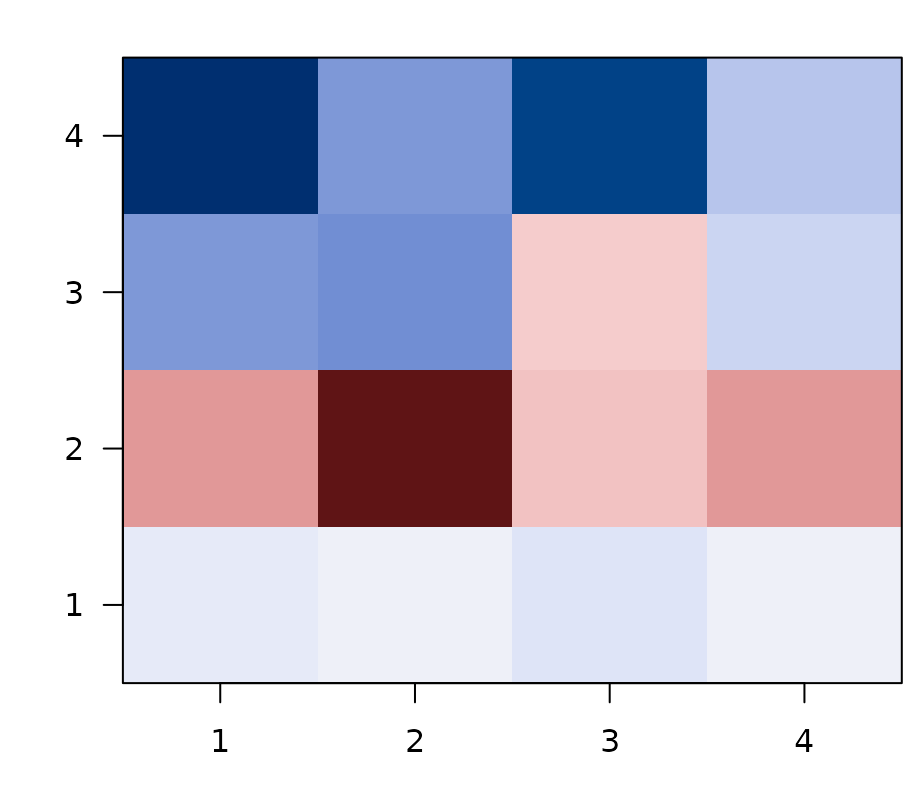
What creates stripes in the ROI x ROI matrix?

Striping usually means one of two things:

• some source ROIs are globally strong predictors of many targets
• some target ROIs are globally easy to predict because they share a large common geometry with many sources

The synthetic example below creates that second pattern on purpose by making some ROIs carry more of a shared representational backbone than others.

stripe_example <- build_striping_example()

knitr::kable(round(stripe_example$raw, 2))

1	2	3	4
1.00	0.92	0.91	0.21
0.90	0.99	0.74	0.21
0.85	0.73	1.00	-0.05
0.29	0.30	0.08	0.99

In the raw matrix, ROIs 1 and 2 are easy targets across the board, while ROI 4 is globally harder. That is the kind of vertical stripe pattern you often see when a common geometry dominates the matrix.

How do the adjustment options differ?

adjust = "double_center" removes additive row and column main effects from the ROI x ROI matrix itself. It is the clean default when you want pair-specific transfer after discounting globally strong sources and globally easy targets.

knitr::kable(round(stripe_example$double_centered, 2))

1	2	3	4
0.11	0.06	0.10	-0.26
0.06	0.17	-0.02	-0.21
0.09	-0.01	0.31	-0.40
-0.26	-0.22	-0.39	0.87

knitr::kable(stripe_example$offsets, digits = 2)

roinum	source_offset	target_offset
1	0.13	0.13
2	0.08	0.11
3	0.00	0.05
4	-0.21	-0.29

The source_offset and target_offset columns quantify the striping directly. Positive source offsets mark ROIs that predict many targets well. Positive target offsets mark ROIs that are easy to predict from many sources.

adjust = "residualize_mean" takes a different approach. It removes the grand-mean RDM component before the cross-correlation is computed, which is better when the stripe pattern reflects one dominant shared geometry present in nearly every ROI.

knitr::kable(round(stripe_example$residualized, 2))

1	2	3	4
0.98	0.09	0.39	-0.70
0.13	0.99	-0.34	-0.29
0.38	-0.26	1.00	-0.70
-0.78	-0.40	-0.74	1.00

Which version should you report?

• Report the raw asymmetric matrix when you want the full descriptive picture, including globally strong sources and globally easy targets.
• Use adjust = "double_center" for visualizations or analyses that are meant to emphasize pair-specific cross-ROI generalization.
• Use adjust = "residualize_mean" when you think a single common geometry is driving much of the matrix and you want to see what remains after removing it.

These adjustments answer different questions, so it is often worth saving both the raw matrix and one adjusted matrix rather than choosing only one.

Feature-RSA vs. model-space connectivity

rMVPA exposes two ways to compute ROI-to-ROI representational connectivity. They are not redundant — they answer subtly different questions, and the right tool depends on whether you supply a model or a feature space:

	Feature-RSA connectivity (this vignette)	Model-space connectivity (vignette("Model_Space_Connectivity"))
What you supply	A feature matrix F (or similarity matrix S)	One or more explicit model RDMs
Fitting	CV-fitted PLS / PCA / glmnet maps neural patterns ↔︎ feature space	No fitting — neural pair vectors are projected onto a fixed model-RDM basis
What gets compared across ROIs	Predicted trial-by-trial RDM vectors (length n_pairs)	Whitened projections onto the model-RDM subspace (length K, the number of model RDMs after orthogonalisation)
Sensitive to	All representational geometry the feature space can capture, including structure beyond the supplied features	Only structure within the declared model-RDM subspace
Memory per ROI	O(n_pairs); often hundreds of thousands of numbers	O(K); typically 2–10 numbers
Best when	You don’t have a clean theoretical RDM; you want a data-driven, model-free similarity measure	You have specific theoretical RDMs (semantic, visual, motor…) and want to ask which regions express each
Diagonal of the connectivity matrix	ROI’s CV-predicted-vs-observed RDM alignment	ROI’s strength of model-RDM expression
Cross-domain pairs (set A vs set B)	Implicit through cross-validated prediction	First-class via pair_rsa_design(..., pairs = "between")

A useful rule of thumb: declared model → model-space connectivity; learned model → feature-RSA connectivity. When in doubt, run both: they make different statistical commitments, and where they disagree is often the most interesting result.

Next steps

If your transfer problem is across cognitive states rather than across ROIs, see vignette("Feature_RSA_Domain_Adaptation"). If you want the broader decision map for within-ROI fits, cross-state transfer, and ROI-to-ROI generalization, see vignette("Feature_RSA_Advanced_Workflows"). For the model-RDM-driven counterpart of the connectivity workflow, see vignette("Model_Space_Connectivity").